13 Summary of Instance-level Exploration
13.1 Introduction
In Part II of the book, we introduced a number of techniques for exploration and explanation of a model’s predictions for individual instances. Each chapter was devoted to a single technique. In practice, these techniques are rarely used separately. Rather, it is more informative to combine different insights offered by each technique into a more holistic overview.
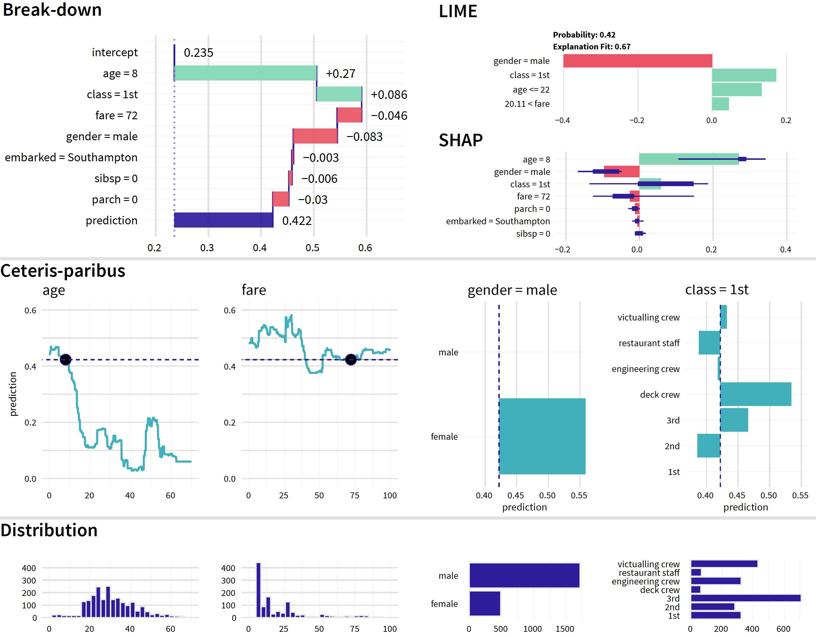
Figure 13.1 offers a graphical illustration of the idea. The graph includes results of four different instance-level explanation techniques applied to the random forest model (Section 4.2.2) for the Titanic data (Section 4.1). The instance of interest is Johnny D, an 8-year-old boy who embarked in Southampton and travelled in the first class with no parents nor siblings, and with a ticket costing 72 pounds (Section 4.2.5). Recall that the goal is to predict the probability of survival of Johnny D.
The plots in the first row of Figure 13.1 show results of application of various variable-attribution and variable-importance methods like break-down (BD) plots (Chapter 6), Shapley values (Chapter 8), and local interpretable model-agnostic explanations (LIME, see Chapter 9). The results consistently suggest that the most important explanatory variables, from a point of view of prediction of the probability of survival for Johnny D, are age, gender, class, and fare. Note, however, that the picture offered by the additive decompositions may not be entirely correct, because fare and class are correlated, and there may be an interaction between the effects of age and gender.
The plots in the second row of Figure 13.1 show ceteris-paribus (CP) profiles (see Chapter 10) for these four most important explanatory variables for Johnny D. The profiles suggest that increasing age or changing the travel class to the second class or to “restaurant staff” would decrease the predicted probability of survival. On the other hand, decreasing the ticket fare, changing gender to female, or changing the travel class to “deck crew” would increase the probability.
The plots in the third row of Figure 13.1 summarize univariate distributions of the four explanatory variables. We see, for instance, that the ticket fare of 72 pounds, which was paid for Johnny D’s ticket, was very high and that there were few children among the passengers of Titanic.
Figure 13.1 nicely illustrates that perspectives offered by the different techniques complement each other and, when combined, allow obtaining a more profound insight into the origins of the model’s prediction for the instance of interest.

Figure 13.1: Results of instance-level-explanation techniques for the random forest model for the Titanic data and passenger Johnny D.
While combining various techniques for instance-level explanation can provide additional insights, it is worth remembering that the techniques are, indeed, different and their suitability may depend on the problem at hand. This is what we discuss in the remainder of the chapter.
13.2 Number of explanatory variables in the model
One of the most important criteria for selection of the exploration and explanation methods is the number of explanatory variables in the model.
13.2.1 Low to medium number of explanatory variables
A low number of variables usually implies that the particular variables have a very concrete meaning and interpretation. An example are variables used in models for the Titanic data presented in Sections 4.2.1 and 4.2.3.
In such a situation, the most detailed information about the influence of the variables on a model’s predictions is provided by the CP profiles. In particular, the variables that are most influential for the model’s predictions are selected by considering CP-profile oscillations (see Chapter 11) and then illustrated graphically with the help of individual-variable CP profiles (see Chapter 10).
13.2.2 Medium to a large number of explanatory variables
In models with a medium or large number of variables, it is still possible that most (or all) of them are interpretable. An example of such a model is a car-insurance pricing model in which we want to estimate the value of an insurance based on behavioral data that includes 100+ variables about characteristics of the driver and characteristics of the car.
When the number of explanatory variables increases, it becomes harder to show the CP profile for each individual variable. In such situations, the most common approach is to use BD plots, presented in Chapter 6, or plots of Shapley values, discussed in Chapter 8. They allow a quick evaluation whether a particular variable has got a positive or negative effect on a model’s prediction; we can also assess the size of the effect. If necessary, it is possible to limit the plots only to the variables with the largest effects.
13.2.3 Very large number of explanatory variables
When the number of explanatory variables is very large, it may be difficult to interpret the role of each single variable. An example of such situations are models for processing of images or texts. In that case, explanatory variables may be individual pixels in image processing or individual characters in text analysis. As such, their individual interpretation is limited. Due to additional issues with computational complexity, it is not feasible to use CP profiles, BD plots, nor Shapley values to evaluate influence of individual values on a model’s predictions. Instead, the most common approach is to use LIME, presented in Chapter 9, which works on the context-relevant groups of variables.
13.4 Models with interactions
In models with interactions, the effect of one explanatory variable may depend on values of other variables. For example, the probability of survival for Titanic passengers may decrease with age, but the effect may be different for different travel-classes.
In such a case, to explore and explain a model’s predictions, we have got to consider not individual variables, but sets of variables included in interactions. To identify interactions, we can use iBD plots, as described in Chapter 7. To show effects of interaction, we may use a set of CP profiles. In particular, for the Titanic example, we may use the CP profiles for the age variable for instances that differ only in gender. The less parallel are such profiles, the larger the effect of interaction.
13.5 Sparse explanations
Predictive models may use hundreds of explanatory variables to yield a prediction for a particular instance. However, for a meaningful interpretation and illustration, most human beings can handle only a very limited (say, less than 10) number of variables. Thus, sparse explanations are of interest. The most common method that is used to construct such explanations is LIME (Chapter 9). However, constructing a sparse explanation for a complex model is not trivial and may be misleading. Hence, care is needed when applying LIME to very complex models.
13.6 Additional uses of model exploration and explanation
In the previous chapters of Part II of the book, we focused on the application of the presented methods to exploration and explanation of predictive models. However, the methods can also be used for other purposes:
Model improvement/debugging. If a model’s prediction is particularly bad for a selected observation, then the investigation of the reasons for such a bad performance may provide hints about how to improve the model. In the case of instance predictions, it is easier to detect that a selected explanatory variable should have a different effect than the observed one.
Additional domain-specific validation. Understanding which factors are important for a model’s predictions helps in evaluation of the plausibility of the model. If the effects of some explanatory variables on the predictions are observed to be inconsistent with the domain knowledge, this may provide a ground for criticising the model and, eventually, replacing it by another one. On the other hand, if the influence of the variables on the model’s predictions is consistent with prior expectations, the user may become more confident with the model. Such confidence is fundamental when the model’s predictions are used as a support for taking decisions that may lead to serious consequences, like in the case of, for example, predictive models in medicine.
Model selection. In the case of multiple candidate models, one may use results of the model explanation techniques to select one of the candidates. It is possible that, even if two models are similar in terms of overall performance, one of them may perform much better locally. Consider the following, highly hypothetical example. Assume that a model is sought to predict whether it will rain on a particular day in a region where it rains on half of the days. Two models are considered: one which simply predicts that it will rain every other day, and another that predicts that it will rain every day since October till March. Arguably, both models are rather unsophisticated (to say the least), but they both predict that, on average, half of the days will be rainy. (We can say that both models are well-calibrated; see Section 15.2.) However, investigation of the instance predictions (for individual days) may lead to a preference for one of them.
New knowledge extraction. Machine-learning models are mainly built for the effectiveness of predictions. As mentioned by Leo Breiman (2001b), it is a different style than the modelling based on the understanding of the phenomena that generated observed values of interests. However, model explanations may sometimes help to extract new and useful knowledge in the field, especially in areas where there is not much domain knowledge yet.
13.7 Comparison of models (champion-challenger analysis)
The techniques for explaining and exploring models have many applications. One of them is the opportunity to compare models.
There are situations when we may be interested in the “champion-challenger” analysis. Let us assume that some institution uses a predictive model, but wants to know if it could get a better model using other modelling techniques. For example, the risk department in a bank may be using logistic regression to assess credit risk. The model may perform satisfactorily and, hence, be considered as the “champion”, i.e., the best model in the class of logistic regression models. However, the department may be interested in checking whether a “challenger”, i.e., a more complex model developed by using, for instance, boosting or random trees, will not perform better. And if it is performing better, the question of interest is: how does the challenger differ from the champion?
Another reason why we may want to compare models is the fact that the modelling process is iterative itself (see Section 2.2). During the process many versions of models are created, often with different structures, and sometimes with a very similar performance. Comparative analysis allows for better understanding of how these models differ from each other.
Below we present an example of a comparative analysis for the logistic regression model titanic_lmr (Section 4.2.1), random forest model titanic_rf (Section 4.2.2), boosting model of titanic_gbm (Section 4.2.3), and support-vector machine (SVM) model titanic_svm (Section 4.2.4). We consider Johnny D (see Section 4.2.5) as the instance of interest.
Note that the models do importantly differ. The random forest and boosting models are tree-based, with a stepped response (prediction) curve. They are complex due to a large number of trees used for prediction. The logistic regression and SVM models lead to continuous and smooth response curves. Their complexity stems from the fact that the logistic regression model includes spline transformations, while the SVM model uses a non-linear kernel function. The differences result in different predicted values of the probability of survival for Johnny D. In particular, the predicted value of the probability is equal to 0.42, 0.77, 0.66, and 0.22 for the random forest, logistic regression, gradient boosting, and SVM model, respectively (see Section 4.2.5).
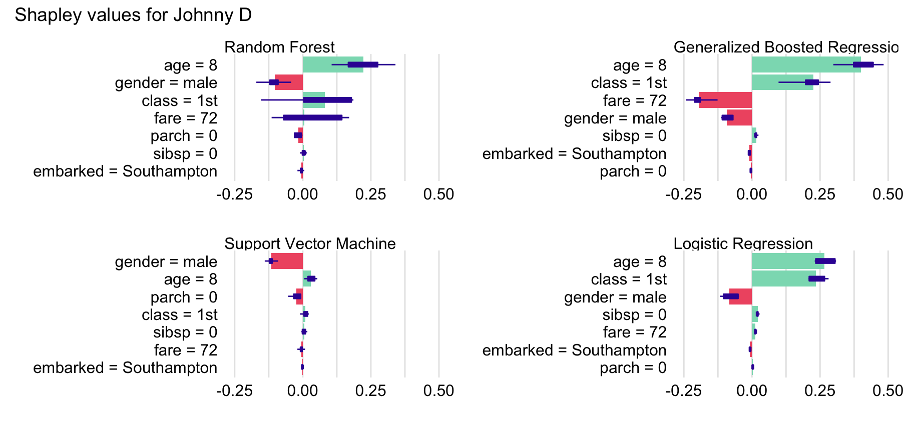
Figure 13.2 shows the Shapley values (see Chapter 8) for the four models for Johnny D. For the random forest and logistic regression models, similar variables are indicated as important: age, class, and gender. Class and gender are also important for the gradient boosting model, while for the SVM model, the most important variable is gender, followed by age and parch.

Figure 13.2: Shapley values for four different models for the Titanic data and passenger Johnny D.
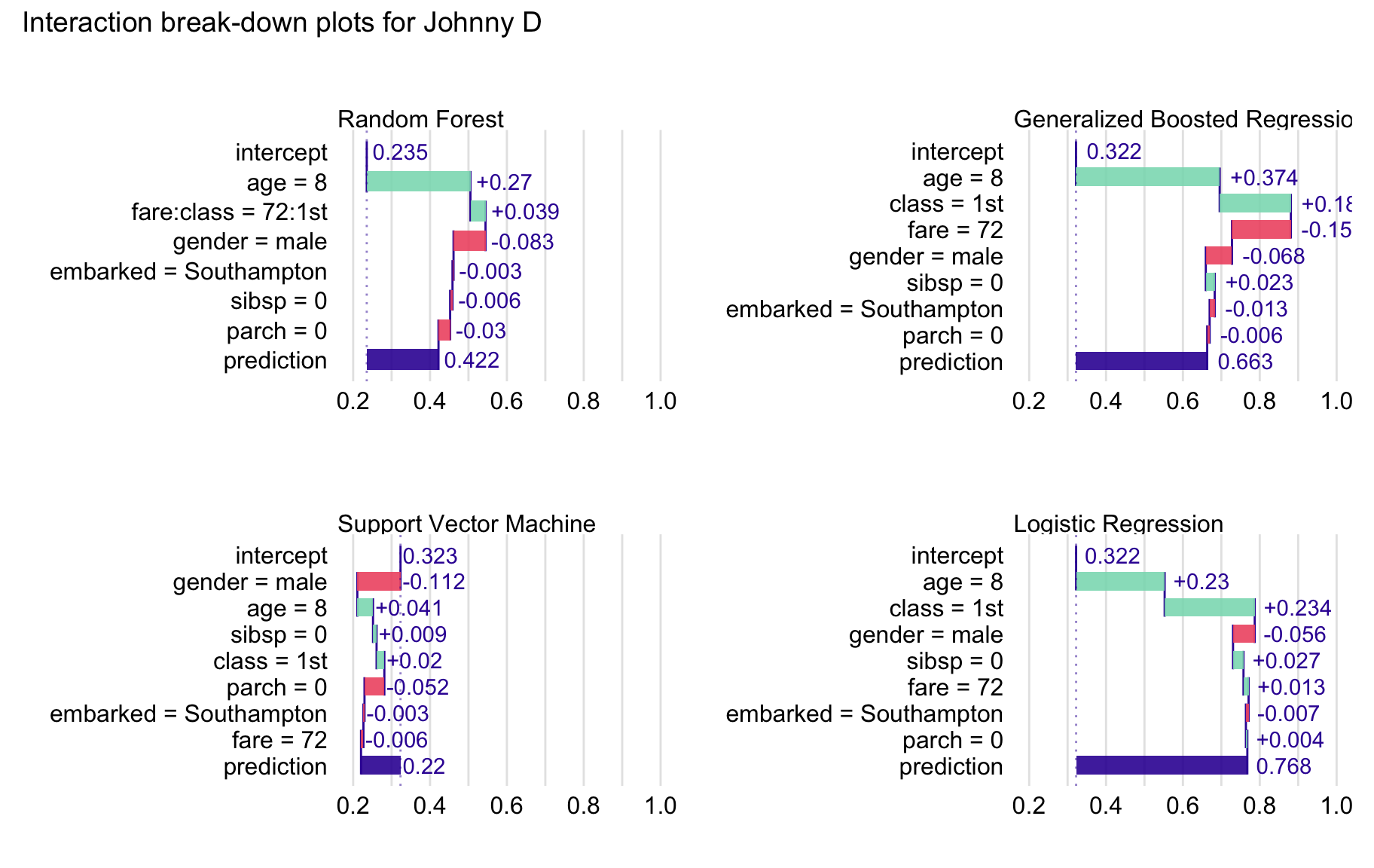
As mentioned in Chapter 8, Shapley values show additive contributions of explanatory variables to a model’s predictions. However, the values may be misleading if there are interactions. In that case, iBD plots, discussed in Chapter 7, might be more appropriate. Figure 13.3 presents the plots for the four models under consideration.
For the SVM model, the most important variable is gender, while for the other models the most important variables are age and class. Remarkably, the iBD plot for the random forest model includes the interaction of fare and class.

Figure 13.3: Interaction break-down plots for four different models for the Titanic data and Johnny D.
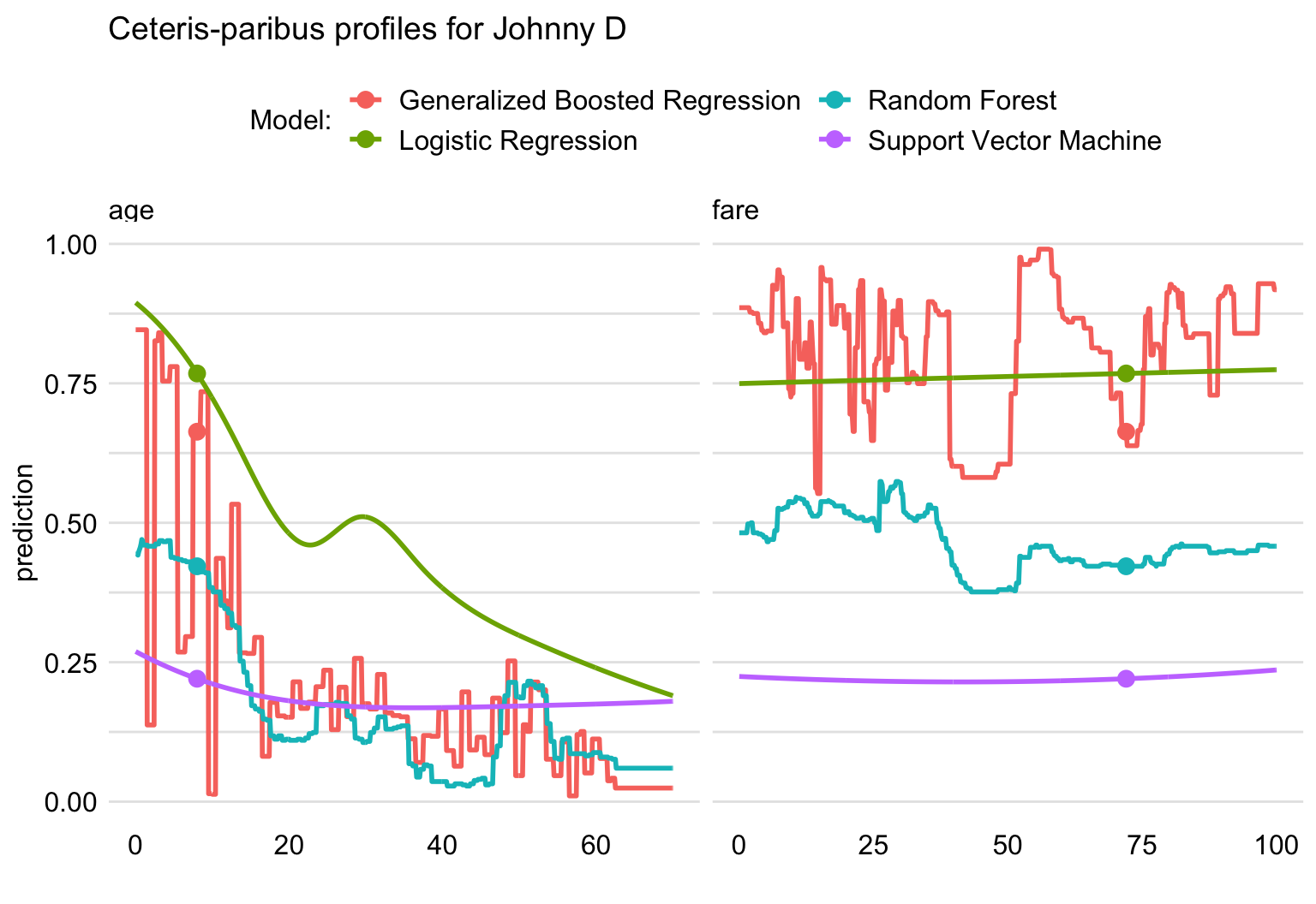
Figure 13.4 shows CP profiles for age and fare and the four compared models. For fare, the logistic regression and SVM models show little effect. A similar conclusion can be drawn for the boosting model, though for this model the profile shows considerable oscillations. The profile for the random forest model suggests a decrease in the predicted probability of survival when the ticket fare increases over about 37 pounds.
For age, the CP profile for the SVM model shows, again, considerable oscillations. For all the models, however, the effect of the variable is substantial, with the predicted probability of survival decreasing with increasing age. The effect is most pronounced for the logistic regression model.

Figure 13.4: Ceteris-paribus plots for variables age and fare for four different models for the Titanic data and passenger Johnny D.
Leo Breiman (2001b) described a phenomenon called “Rashomon effect”. It means that different models with a similar performance can base their predictions on completely different relations extracted from the same data.
This is the case with the four models presented in this chapter. Although they are all quite effective, for one particular observation, Johnny D, they give different predictions and different explanations.
Despite the differences, the explanations are very useful. For example, the CP profiles for the gradient boosting model exhibit high fluctuations (see Figure 13.4). Such fluctuations suggest overfitting, so one might be inclined not to use this model. The CP profiles for age, presented in Figure 13.4, indicate that the SVM model is rather inflexible in that it cannot capture the trend, seen for the remaining three models, that young passengers had a better chance of survival. This could be taken as an argument against the use of the SVM model.
The CP-profiles for the random forest-model are, in general, consistent with the logistic regression model (see Figure 13.4). However, box plots in Figure 13.2 show that explanatory-variable attributions for the random forest model are highly variable. This indicates the presence of interactions in the model. However, for a model with interactions, the additive explanations for individual explanatory variables can be misleading.
Based on this analysis, we might conclude that the most recommendable of the four models is the logistic regression model with splines.
References
Breiman, Leo. 2001b. “Statistical modeling: The two cultures.” Statistical Science 16 (3): 199–231. https://doi.org/10.1214/ss/1009213726.