4 Datasets and Models
We will illustrate the methods presented in this book by using three datasets related to:
- predicting probability of survival for passengers of the RMS Titanic;
- predicting prices of apartments in Warsaw;
- predicting the value of the football players based on the FIFA dataset.
The first dataset will be used to illustrate the application of the techniques in the case of a predictive (classification) model for a binary dependent variable. It is mainly used in the examples presented in the second part of the book. The second dataset will be used to illustrate the exploration of prediction models for a continuous dependent variable. It is mainly used in the examples in the third part of this book. The third dataset will be introduced in Chapter 21 and will be used to illustrate the use of all of the techniques introduced in the book.
In this chapter, we provide a short description of the first two datasets, together with results of exploratory analyses. We also introduce models that will be used for illustration purposes in subsequent chapters.
4.1 Sinking of the RMS Titanic
The sinking of the RMS Titanic is one of the deadliest maritime disasters in history (during peacetime). Over 1500 people died as a consequence of a collision with an iceberg. Projects like Encyclopedia titanica (https://www.encyclopedia-titanica.org/) are a source of rich and precise data about Titanic’s passengers.
The stablelearner package in R includes a data frame with information about passengers’ characteristics. The dataset, after some data cleaning and variable transformations, is also available in the DALEX package for R and in the dalex library for Python. In particular, the titanic data frame contains 2207 observations (for 1317 passengers and 890 crew members) and nine variables:
- gender, person’s (passenger’s or crew member’s) gender, a factor (categorical variable) with two levels (categories): “male” (78%) and “female” (22%);
- age, person’s age in years, a numerical variable; the age is given in (integer) years, in the range of 0–74 years;
- class, the class in which the passenger travelled, or the duty class of a crew member; a factor with seven levels: “1st” (14.7%), “2nd” (12.9%), “3rd” (32.1%), “deck crew” (3%), “engineering crew” (14.7%), “restaurant staff” (3.1%), and “victualling crew” (19.5%);
- embarked, the harbor in which the person embarked on the ship, a factor with four levels: “Belfast” (8.9%), “Cherbourg” (12.3%), “Queenstown” (5.6%), and “Southampton” (73.2%);
- country, person’s home country, a factor with 48 levels; the most common levels are “England” (51%), “United States” (12%), “Ireland” (6.2%), and “Sweden” (4.8%);
- fare, the price of the ticket (only available for passengers; 0 for crew members), a numerical variable in the range of 0–512;
- sibsp, the number of siblings/spouses aboard the ship, a numerical variable in the range of 0–8;
- parch, the number of parents/children aboard the ship, a numerical variable in the range of 0–9;
- survived, a factor with two levels: “yes” (67.8%) and “no” (32.2%) indicating whether the person survived or not.
The first six rows of this dataset are presented in the table below.
| gender | age | class | embarked | fare | sibsp | parch | survived |
|---|---|---|---|---|---|---|---|
| male | 42 | 3rd | Southampton | 7.11 | 0 | 0 | no |
| male | 13 | 3rd | Southampton | 20.05 | 0 | 2 | no |
| male | 16 | 3rd | Southampton | 20.05 | 1 | 1 | no |
| female | 39 | 3rd | Southampton | 20.05 | 1 | 1 | yes |
| female | 16 | 3rd | Southampton | 7.13 | 0 | 0 | yes |
| male | 25 | 3rd | Southampton | 7.13 | 0 | 0 | yes |
Models considered for this dataset will use survived as the (binary) dependent variable.
4.1.1 Data exploration
As discussed in Chapter 2, it is always advisable to explore data before modelling. However, as this book is focused on model exploration, we will limit the data exploration part.
Before exploring the data, we first conduct some pre-processing. In particular, the value of variables age, country, sibsp, parch, and fare is missing for a limited number of observations (2, 81, 10, 10, and 26, respectively). Analyzing data with missing values is a topic on its own (Schafer 1997; Little and Rubin 2002; Molenberghs and Kenward 2007). An often-used approach is to impute the missing values. Toward this end, multiple imputations should be considered (Schafer 1997; Molenberghs and Kenward 2007; Buuren 2012). However, given the limited number of missing values and the intended illustrative use of the dataset, we will limit ourselves to, admittedly inferior, single imputation. In particular, we replace the missing age values by the mean of the observed ones, i.e., 30. Missing country is encoded by "X". For sibsp and parch, we replace the missing values by the most frequently observed value, i.e., 0. Finally, for fare, we use the mean fare for a given class, i.e., 0 pounds for crew, 89 pounds for the first, 22 pounds for the second, and 13 pounds for the third class.
After imputing the missing values, we investigate the association between survival status and other variables. Most variables in the Titanic dataset are categorical, except of age and fare. Figure 4.1 shows histograms for the latter two variables. In order to keep the exploration uniform, we transform the two variables into categorical ones. In particular, age is discretized into five categories by using cutoffs equal to 5, 10, 20, and 30, while fare is discretized by applying cutoffs equal to 1, 10, 25, and 50.
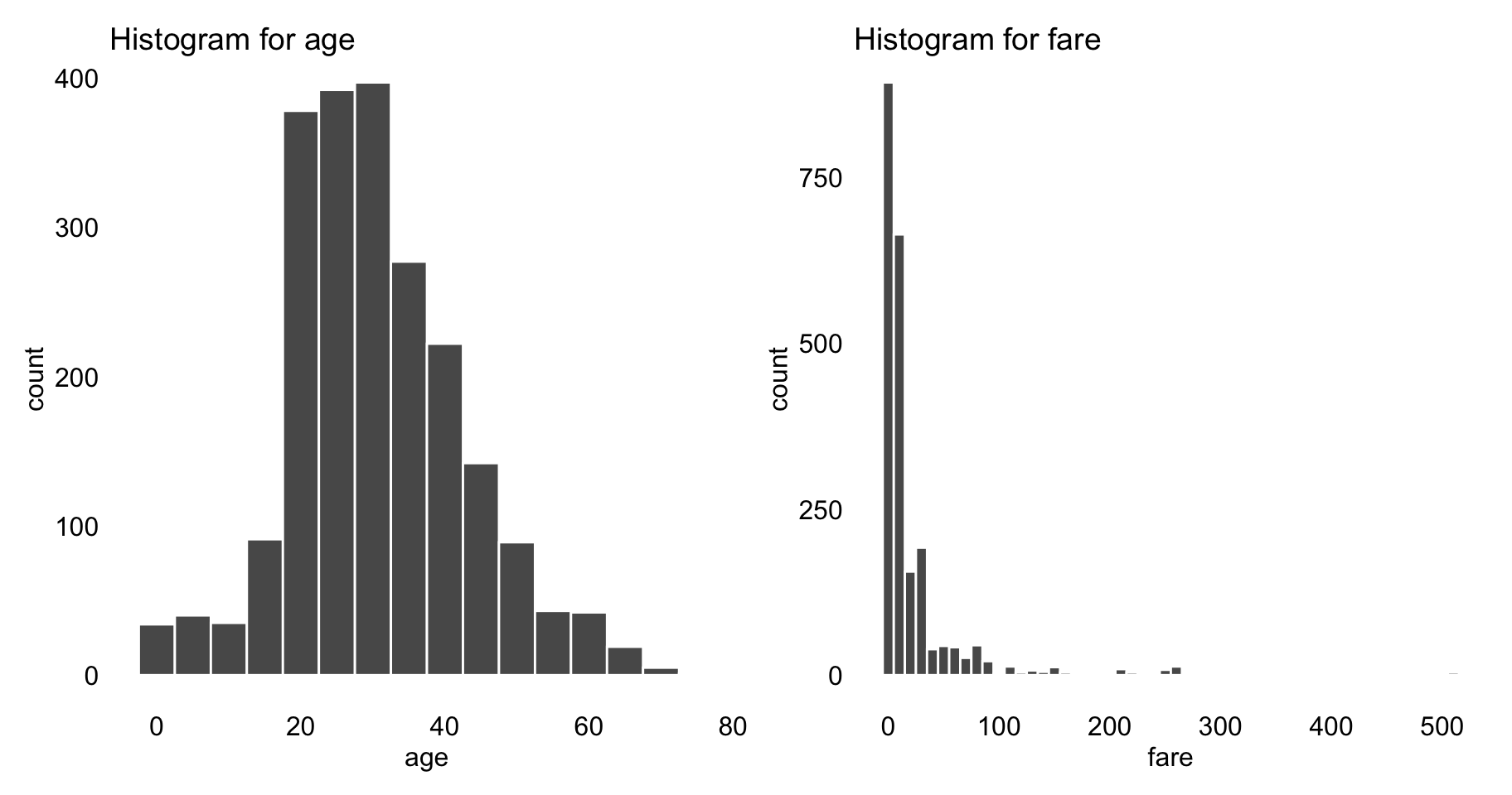
Figure 4.1: Histograms for variables age and fare from the Titanic data.
Figures 4.2–4.5 present graphically, with the help of mosaic plots, the proportion of non- and survivors for different levels of other variables. The width of the bars (on the x-axis) reflects the marginal distribution (proportions) of the observed levels of the variable. On the other hand, the height of the bars (on the y-axis) provides information about the proportion of non- and survivors. The graphs for age and fare were constructed by using the categorized versions of the variables.
Figure 4.2 indicates that the proportion of survivors was larger for females and children below 5 years of age. This is most likely the result of the “women and children first” principle that is often evoked in situations that require the evacuation of persons whose life is in danger.
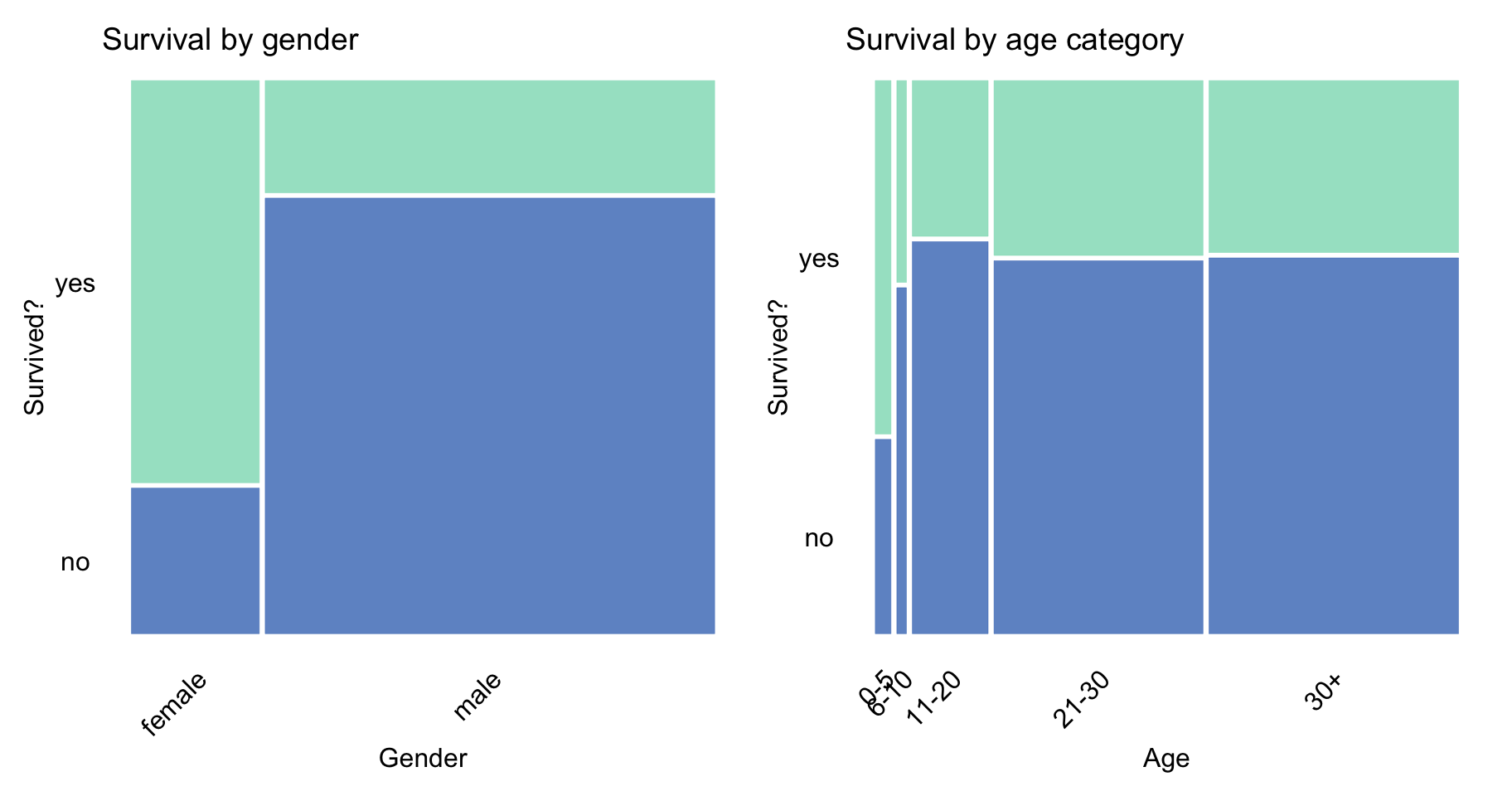
Figure 4.2: Survival according to gender and age category in the Titanic data.
The principle can, perhaps, partially explain the trend seen in Figure 4.3, i.e., a higher proportion of survivors among those with 1-2 parents/children and 1-2 siblings/spouses aboard.
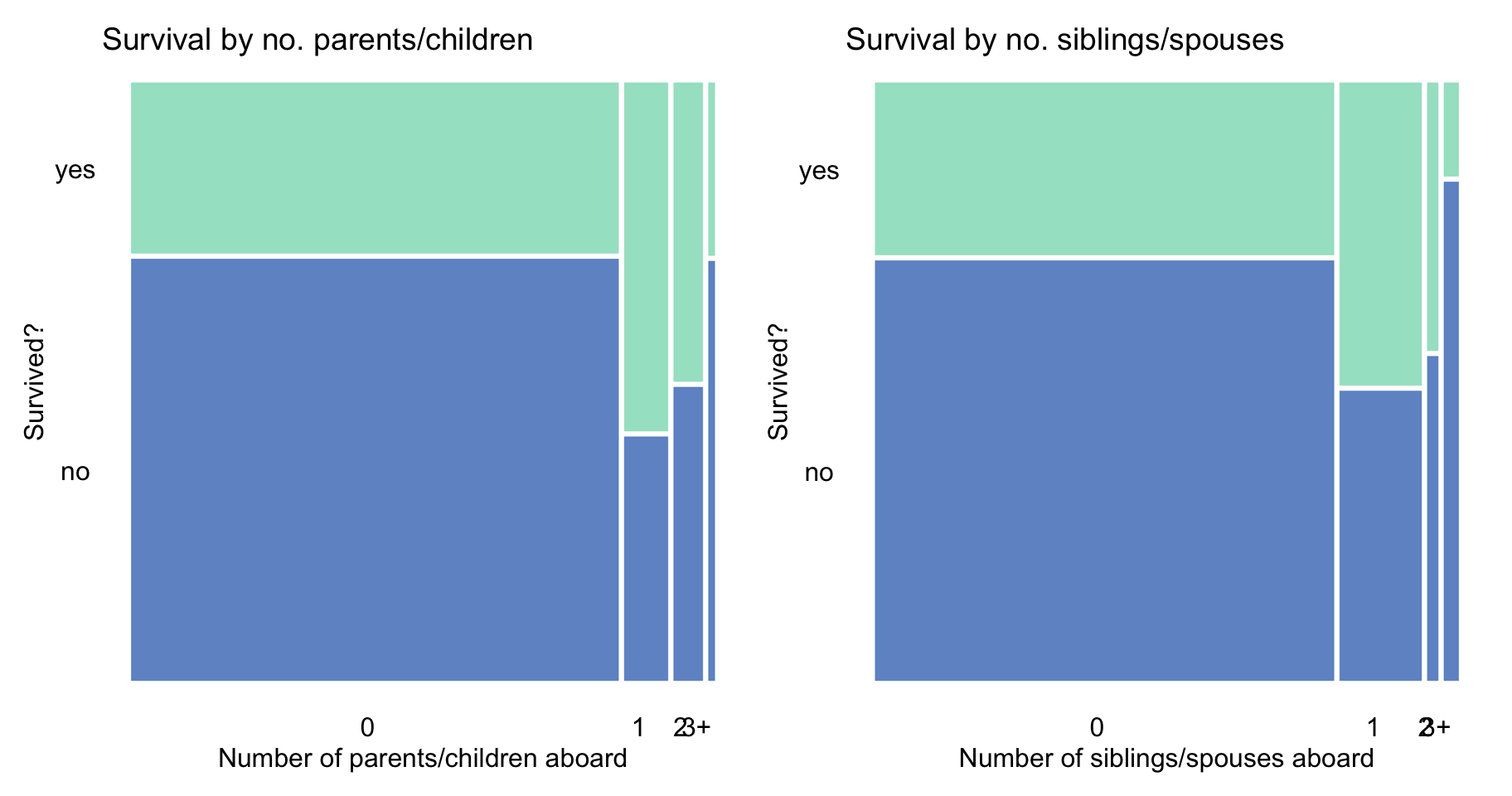
Figure 4.3: Survival according to the number of parents/children and siblings/spouses in the Titanic data.
Figure 4.4 indicates that passengers travelling in the first and second class had a higher chance of survival, perhaps due to the proximity of the location of their cabins to the deck. Interestingly, the proportion of survivors among the deck crew was similar to the proportion of the first-class passengers. The figure also shows that the proportion of survivors increased with the fare, which is consistent with the fact that the proportion was higher for passengers travelling in the first and second class.
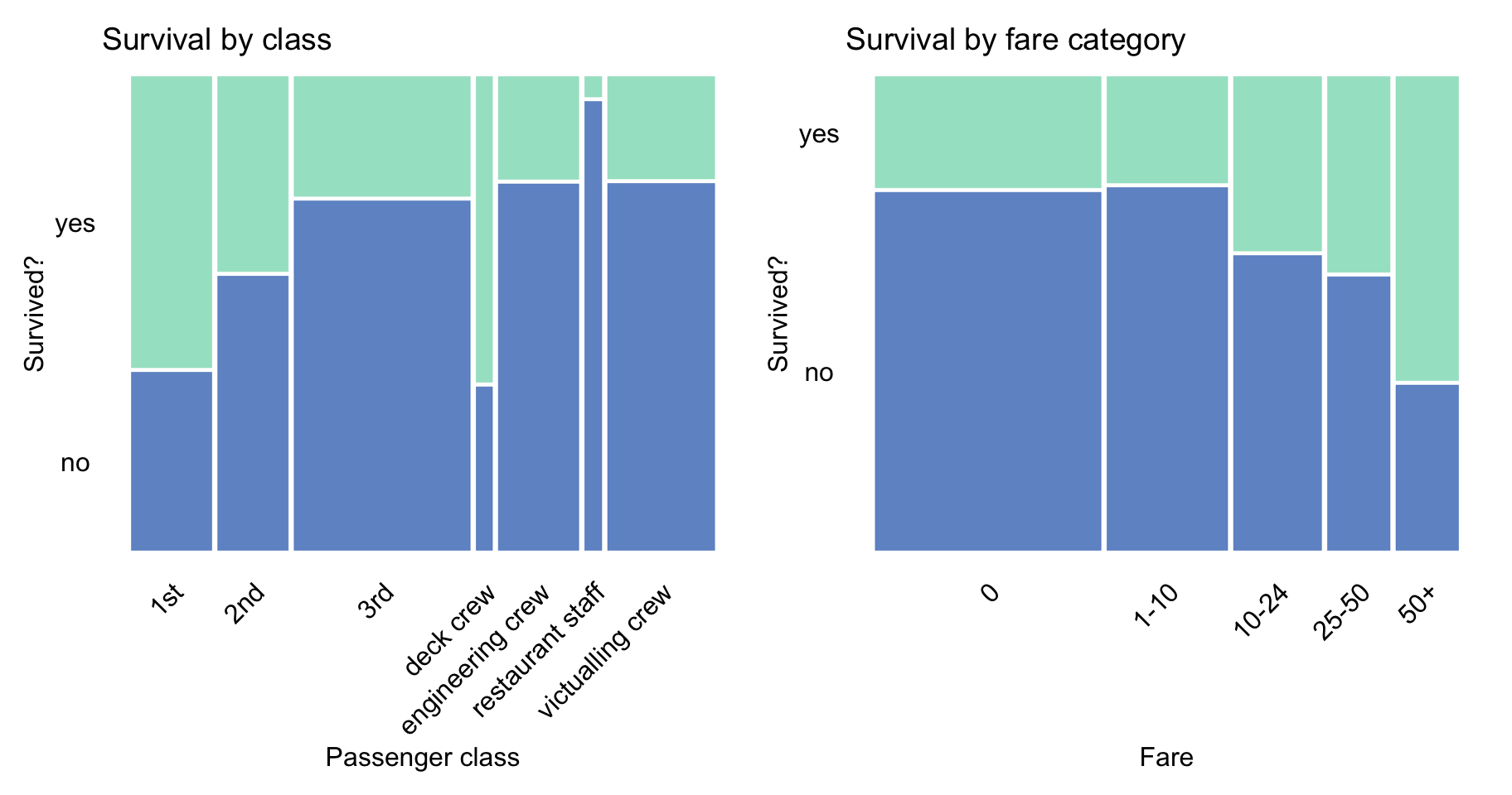
Figure 4.4: Survival according to travel-class and ticket-fare in the Titanic data.
Finally, Figure 4.5 does not suggest any noteworthy trends.
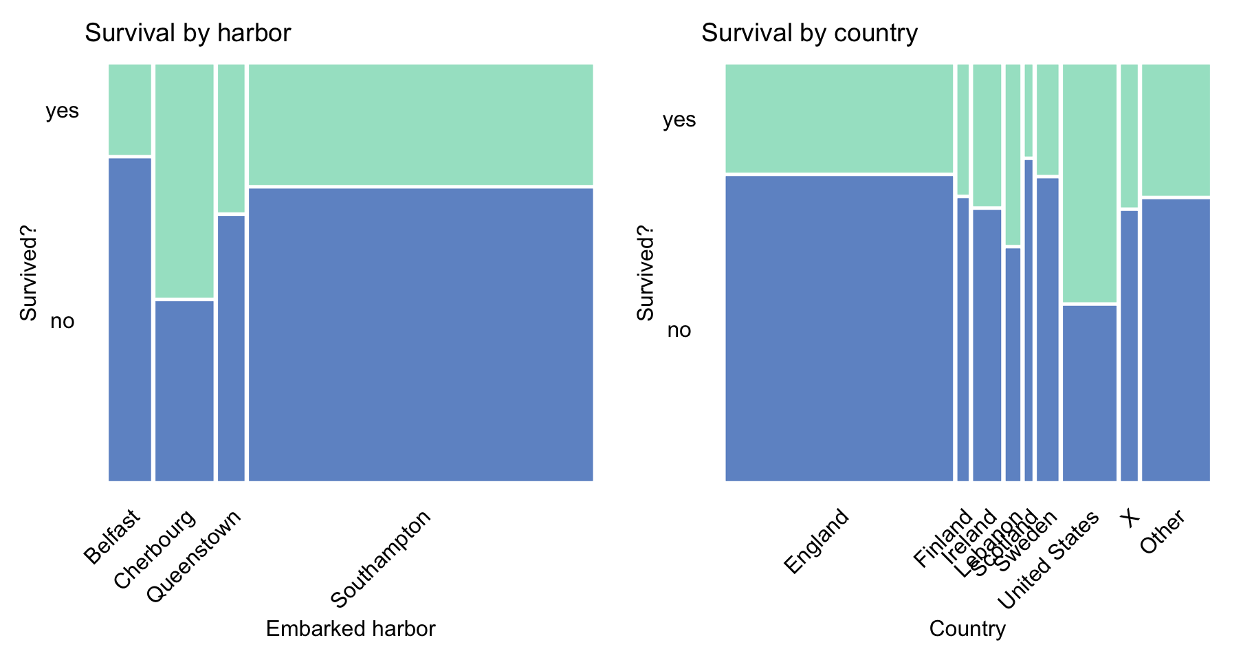
Figure 4.5: Survival according to the embarked harbour and country in the Titanic data.
4.2 Models for RMS Titanic, snippets for R
4.2.1 Logistic regression model
The dependent variable of interest, survived, is binary. Thus, a natural choice is to start the predictive modelling with a logistic regression model. As there is no reason to expect a linear relationship between age and odds of survival, we use linear tail-restricted cubic splines, available in the rcs() function of the rms package (Harrell Jr 2018), to model the effect of age. We also do not expect linear relation for the fare variable, but because of its skewness (see Figure 4.1), we do not use splines for this variable. The results of the model are stored in model-object titanic_lmr, which will be used in subsequent chapters.
library("rms")
titanic_lmr <- lrm(survived == "yes" ~ gender + rcs(age) + class +
         sibsp + parch + fare + embarked, titanic)
Note that we are not very much interested in the assessment of the model’s predictive performance, but rather on understanding how the model yields its predictions. This is why we do not split the data into the training and testing subsets. Instead, the model is fitted to the entire dataset and will be examined on the same dataset.
4.2.2 Random forest model
As an alternative to the logistic regression model we consider a random forest model. Random forest modelling is known for good predictive performance, ability to grasp low-order variable interactions, and stability (Leo Breiman 2001a). To fit the model, we apply the randomForest() function, with default settings, from the package with the same name (Liaw and Wiener 2002). In particular, we fit a model with the same set of explanatory variables as the logistic regression model (see Section 4.2.1). The results of the random forest model are stored in model-object titanic_rf.
4.2.3 Gradient boosting model
Additionally, we consider the gradient boosting model (Friedman 2000). Tree-based boosting models are known for being able to accommodate higher-order interactions between variables. We use the same set of six explanatory variables as for the logistic regression model (see Section 4.2.1). To fit the gradient boosting model, we use function gbm() from the gbm package (Ridgeway 2017). The results of the model are stored in model-object titanic_gbm.
4.2.4 Support vector machine model
Finally, we also consider a support vector machine (SVM) model (Cortes and Vapnik 1995). We use the C-classification mode. Again, we fit a model with the same set of explanatory variables as in the logistic regression model (see Section 4.2.1) To fit the model, we use function svm() from the e1071 package (Meyer et al. 2019). The results of the model are stored in model-object titanic_svm.
4.2.5 Models’ predictions
Let us now compare predictions that are obtained from the different models. In particular, we compute the predicted probability of survival for Johnny D, an 8-year-old boy who embarked in Southampton and travelled in the first class with no parents nor siblings, and with a ticket costing 72 pounds.
First, we create a data frame johnny_d that contains the data describing the passenger.
johnny_d <- data.frame(
          class = factor("1st", levels = c("1st", "2nd", "3rd",
                     "deck crew", "engineering crew",
                     "restaurant staff", "victualling crew")),
          gender = factor("male", levels = c("female", "male")),
          age = 8, sibsp = 0, parch = 0, fare = 72,
          embarked = factor("Southampton", levels = c("Belfast",
                      "Cherbourg","Queenstown","Southampton")))
Subsequently, we use the generic function predict() to obtain the predicted probability of survival for the logistic regression model.
##         1
## 0.7677036
The predicted probability is equal to 0.77.
We do the same for the remaining three models.
##      no   yes
## 1 0.578 0.422
## attr(,"class")
## [1] "matrix" "array" "votes"## [1] 0.6632574## 1
## FALSE
## attr(,"probabilities")
## FALSE TRUE
## 1 0.7799685 0.2200315
## Levels: FALSE TRUEAs a result, we obtain the predicted probabilities of 0.42, 0.66, and 0.22 for the random forest, gradient boosting, and SVM models, respectively. The models lead to different probabilities. Thus, it might be of interest to understand the reason for the differences, as it could help us decide which of the predictions we might want to trust. We will investigate this issue in the subsequent chapters.
Note that, for some examples later in the book, we will use another observation (instance). We will call this passenger Henry.
henry <- data.frame(
       class = factor("1st", levels = c("1st", "2nd", "3rd",
                  "deck crew", "engineering crew",
                  "restaurant staff", "victualling crew")),
       gender = factor("male", levels = c("female", "male")),
       age = 47, sibsp = 0, parch = 0, fare = 25,
       embarked = factor("Cherbourg", levels = c("Belfast",
                         "Cherbourg","Queenstown","Southampton")))
For Henry, the predicted probability of survival is lower than for Johnny D.
##         1
## 0.4318245## [1] 0.246## [1] 0.3073358## [1] 0.17679954.2.6 Models’ explainers
Model-objects created with different libraries may have different internal structures. Thus, first, we have got to create an “explainer,” i.e., an object that provides an uniform interface for different models. Toward this end, we use the explain() function from the DALEX package (Biecek 2018). As it was mentioned in Section 3.1.2, there is only one argument that is required by the function, i.e., model. The argument is used to specify the model-object with the fitted form of the model. However, the function allows additional arguments that extend its functionalities. In particular, the list of arguments includes the following:
data, a data frame or matrix providing data to which the model is to be applied; if not provided (data = NULLby default), the data are extracted from the model-object. Note that the data object should not, in principle, contain the dependent variable.y, observed values of the dependent variable corresponding to the data given in thedataobject; if not provided (y = NULLby default), the values are extracted from the model-object;predict_function, a function that returns prediction scores; if not specified (predict_function = NULLby default), then a defaultpredict()function is used (note that this may lead to errors);residual_function, a function that returns model residuals; if not specified (residual_function = NULLby default), then model residuals defined in equation (2.1) are calculated;verbose, a logical argument (verbose = TRUEby default) indicating whether diagnostic messages are to be printed;precalculate, a logical argument (precalculate = TRUEby default) indicating whether predicted values and residuals are to be calculated when the explainer is created. Note that this will also happen ifverbose = TRUE. To skip the calculations, bothverboseandprecalculateshould be set to FALSE .model_info, a named list (with componentspackage,version, andtype) providing information about the model; if not specified (model_info = NULLby default),DALEXseeks for information on its own;type, information about the type of the model, either"classification"(for a binary dependent variable) or"regression"(for a continuous dependent variable); if not specified (type = NULLby default), then the value of the argument is extracted frommodel_info;label, a unique name of the model; if not specified (label = NULLby default), then it is extracted fromclass(model).
Application of function explain() provides an object of class explainer. It is a list of many components that include:
model, the explained model;data, the data to which the model is applied;y, observed values of the dependent variable corresponding todata;y_hat, predictions obtained by applyingmodeltodata;residuals, residuals computed based onyandy_hat;predict_function, the function used to obtain the model’s predictions;residual_function, the function used to obtain residuals;class, class/classes of the model;label, label of the model/explainer;model_info, a named list (with componentspackage,version, andtype) providing information about the model.
Thus, each explainer-object contains all elements needed to create a model explanation. The code below creates explainers for the models (see Sections 4.2.1–4.2.4) fitted to the Titanic data. Note that, in the data argument, we indicate the titanic data frame without the ninth column, i.e., without the survived variable. The variable is used in the y argument to explicitly define the binary dependent variable equal to 1 for survivors and 0 for passengers who did not survive.
titanic_lmr_exp <- explain(model = titanic_lmr,
                       data = titanic[, -9],
                       y = titanic$survived == "yes",
                       label = "Logistic Regression",
                       type = "classification")
titanic_rf_exp <- explain(model = titanic_rf,
                       data = titanic[, -9],
                       y = titanic$survived == "yes",
                       label = "Random Forest")
titanic_gbm_exp <- explain(model = titanic_gbm,
                       data = titanic[, -9],
                       y = titanic$survived == "yes",
                       label = "Generalized Boosted Regression")
titanic_svm_exp <- explain(model = titanic_svm,
                       data = titanic[, -9],
                       y = titanic$survived == "yes",
                       label = "Support Vector Machine")
4.2.7 List of model-objects
In the previous sections, we have built four predictive models for the Titanic dataset. The models will be used in the rest of the book to illustrate model-explanation methods and tools.
For the ease of reference, we summarize the models in Table 4.1. The binary model-objects can be downloaded by using the indicated archivist hooks (Biecek and Kosinski 2017). By calling a function specified in the last column of the table, one can restore a selected model in its local R environment.
| Model name / library | Link to this object |
|---|---|
titanic_lmr |
Get the model: archivist:: |
rms:: lmr v.5.1.3 |
aread("pbiecek/models/58b24"). |
titanic_rf |
Get the model: archivist:: |
randomForest:: randomForest v.4.6.14 |
aread("pbiecek/models/4e0fc"). |
titanic_gbm |
Get the model: archivist:: |
gbm:: gbm v.2.1.5 |
aread("pbiecek/models/b7078"). |
titanic_svm |
Get the model: archivist:: |
e1071:: svm v.1.7.3 |
aread("pbiecek/models/9c27f"). |
Table 4.2 summarizes the data frames that will be used in examples in the subsequent chapters.
| Description | Link to this object |
|---|---|
titanic dataset with 2207 observations with imputed missing values |
archivist:: aread("pbiecek/models/27e5c") |
johnny_d 8-year-old boy from the 1st class without parents, paid 72 pounds, embarked in Southampton |
archivist:: aread("pbiecek/models/e3596") |
henry 47-year-old male from the 1st class, travelled alone, paid 25 pounds, embarked in Cherbourg |
archivist:: aread("pbiecek/models/a6538") |
4.3 Models for RMS Titanic, snippets for Python
Titanic data are provided in the titanic dataset, which is available in the dalex library. The values of the dependent binary variable are given in the survived column; the remaining columns give the values of the explanatory variables that are used to construct the classifiers.
The following instructions load the titanic dataset and split it into the dependent variable y and the explanatory variables X. Note that, for the purpose of this example, we do not divide the data into the training and testing sets. Instructions on how to deal with the situation when you want to analyze the model on data other than the training set will be presented in the subsequent chapters.
import dalex as dx
titanic = dx.datasets.load_titanic()
X = titanic.drop(columns='survived')
y = titanic.survived
Dataset X contains numeric variables with different ranges (for instance, age and fare) and categorical variables. Machine-learning algorithms in the sklearn library require data in a numeric form. Therefore, before modelling, we use a pipeline that performs data pre-processing. In particular, we scale the continuous variables (age, fare, parch, and sibsp) and one-hot-encode the categorical variables (gender, class, embarked).
from sklearn.preprocessing import StandardScaler, OneHotEncoder
from sklearn.compose import make_column_transformer
from sklearn.pipeline import make_pipeline

preprocess = make_column_transformer(
    (StandardScaler(), ['age', 'fare', 'parch', 'sibsp']),
    (OneHotEncoder(), ['gender', 'class', 'embarked']))
4.3.1 Logistic regression model
To fit the logistic regression model (see Section 4.2.1), we use the LogisticRegression algorithm from the sklearn library. By default, the implementation uses the ridge penalty, defined in (2.6). For this reason it is important to scale continuous variables like age and fare.
The fitted model is stored in object titanic_lr, which will be used in subsequent chapters.
4.3.2 Random forest model
To fit the random forest model (see Section 4.2.2), we use the RandomForestClassifier algorithm from the sklearn library. We use the default settings with trees not deeper than three levels, and the number of trees set to 500. The fitted model is stored in object titanic_rf.
4.3.3 Gradient boosting model
To fit the gradient boosting model (see Section 4.2.3), we use the GradientBoostingClassifier algorithm from the sklearn library. We use the default settings, with the number of trees in the ensemble set to 100. The fitted model is stored in object titanic_gbc.
4.3.4 Support vector machine model
Finally, to fit the SVM model with C-Support Vector Classification mode (see Section 4.2.4), we use the SVC algorithm from the sklearn library based on libsvm. The fitted model is stored in object titanic_svm.
4.3.5 Models’ predictions
Let us now compare predictions that are obtained from the different models. In particular, we compute the predicted probability of survival for Johnny D, an 8-year-old boy who embarked in Southampton and travelled in the first class with no parents nor siblings, and with a ticket costing 72 pounds (see Section 4.2.5).
First, we create a data frame johnny_d that contains the data describing the passenger.
import pandas as pd

johnny_d = pd.DataFrame({'gender': ['male'],
                       'age'     : [8],
                       'class'   : ['1st'],
                       'embarked': ['Southampton'],
                       'fare'    : [72],
                       'sibsp'   : [0],
                       'parch'   : [0]},
                      index = ['JohnnyD'])
Subsequently, we use the method predict_proba() to obtain the predicted probability of survival for the logistic regression model.
We do the same for the three remaining models.
titanic_rf.predict_proba(johnny_d)
# array([[0.63028556, 0.36971444]])
titanic_gbc.predict_proba(johnny_d)
# array([[0.1567194, 0.8432806]])
titanic_svm.predict_proba(johnny_d)
# array([[0.78308146, 0.21691854]])
We also create data frame for passenger Henry (see Section 4.2.5) and compute his predicted probability of survival.
henry = pd.DataFrame({'gender'   : ['male'],
                       'age'     : [47],
                       'class'   : ['1st'],
                       'embarked': ['Cherbourg'],
                       'fare'    : [25],
                       'sibsp'   : [0],
                       'parch'   : [0]},
                      index = ['Henry'])
titanic_lr.predict_proba(henry)
# array([[0.56798421 0.43201579]])
titanic_rf.predict_proba(henry)
# array([[0.69917845 0.30082155]])
titanic_gbc.predict_proba(henry)
# array([[0.78542886 0.21457114]])
titanic_svm.predict_proba(henry)
# array([[0.81725832 0.18274168]])
4.3.6 Models’ explainers
The Python-code examples shown above use functions from the sklearn library, which facilitates uniform working with models. However, we may want to, or have to, work with models built by using other libraries. To simplify the task, the dalex library wraps models in objects of class Explainer that contain, in a uniform way, all the functions necessary for working with models.
There is only one argument that is required by the Explainer() constructor, i.e., model. However, the constructor allows additional arguments that extend its functionalities. In particular, the list of arguments includes the following:
data, a data frame ornumpy.ndarrayproviding data to which the model is to be applied. It should be an object of thepandas.DataFrameclass, otherwise it will be converted topandas.DataFrame.y, values of the dependent variable/target variable corresponding to the data given in thedataobject;predict_function, a function that returns prediction scores; if not specified, thendalexwill make a guess which function should be used (predict(),predict_proba(), or something else). Note that this function should work onpandas.DataFrameobjects; if it works only onnumpy.ndarraythen an appropriate conversion should also be included inpredict_function.residual_function, a function that returns model residuals;label, a unique name of the model;model_class, the class of actual model;verbose, a logical argument (verbose = TRUEby default) indicating whether diagnostic messages are to be printed;model_type, information about the type of the model, either"classification"(for a binary dependent variable) or"regression"(for a continuous dependent variable);model_info, a dictionary with additional information about the model.
Application of constructor Explainer() provides an object of class Explainer. It is an object with many components that include:
model, the explained model;data, the data to which the model is applied;y, observed values of the dependent variable corresponding todata;y_hat, predictions obtained by applyingmodeltodata;residuals, residuals computed based onyandy_hat;predict_function, the function used to obtain the model’s predictions;residual_function, the function used to obtain residuals;class, class/classes of the model;label, label of the model/explainer;model_info, a dictionary (with componentspackage,version, andtype) providing information about the model.
Thus, each explainer-object contains all elements needed to create a model explanation. The code below creates explainers for the models (see Sections 4.3.1–4.3.4) fitted to the Titanic data.
titanic_rf_exp = dx.Explainer(titanic_rf,
                    X, y, label = "Titanic RF Pipeline")
titanic_lr_exp = dx.Explainer(titanic_lr,
                    X, y, label = "Titanic LR Pipeline")
titanic_gbc_exp = dx.Explainer(titanic_gbc,
                    X, y, label = "Titanic GBC Pipeline")
titanic_svm_exp = dx.Explainer(titanic_svm,
                    X, y, label = "Titanic SVM Pipeline")
When an explainer is created, the specified model and data are tested for consistency.
Diagnostic information is printed on the screen.
The following output shows diagnostic information for the titanic_rf model.
Preparation of a new explainer is initiated

  -> data              : 2207 rows 7 cols
  -> target variable   : Argument 'y' was converted to a numpy.ndarray.
  -> target variable   : 2207 values
  -> model_class       : sklearn.pipeline.Pipeline (default)
  -> label             : Titanic RF Pipeline
  -> predict function  : <yhat_proba> will be used (default)
  -> predicted values  : min = 0.171, mean = 0.322, max = 0.893
  -> residual function : difference between y and yhat (default)
  -> residuals         : min = -0.826, mean = 4.89e-05, max = 0.826
  -> model_info        : package sklearn

A new explainer has been created!
4.4 Apartment prices
Predicting house prices is a common exercise used in machine-learning courses. Various datasets for house prices are available at websites like Kaggle or UCI Machine Learning Repository.
In this book, we will work with an interesting variant of this problem. The apartments dataset contains simulated data that match key characteristics of real apartments in Warsaw, the capital of Poland. However, the dataset is created in a way that two very different models, namely linear regression and random forest, offer almost exactly the same overall accuracy of predictions. The natural question is then: which model should we choose? We will show that model-explanation tools provide important insight into the key model characteristics and are helpful in model selection.
The dataset is available in the DALEX package in R and the dalex library in Python. It contains 1000 observations (apartments) and six variables:
- m2.price, apartment’s price per square meter (in EUR), a numerical variable in the range of 1607–6595;
- construction.year, the year of construction of the block of flats in which the apartment is located, a numerical variable in the range of 1920–2010;
- surface, apartment’s total surface in square meters, a numerical variable in the range of 20–150;
- floor, the floor at which the apartment is located (ground floor taken to be the first floor), a numerical integer variable with values ranging from 1 to 10;
- no.rooms, the total number of rooms, a numerical integer variable with values ranging from 1 to 6;
- district, a factor with 10 levels indicating the district of Warsaw where the apartment is located.
The first six rows of this dataset are presented in the table below.
| m2.price | construction.year | surface | floor | no.rooms | district |
|---|---|---|---|---|---|
| 5897 | 1953 | 25 | 3 | 1 | Srodmiescie |
| 1818 | 1992 | 143 | 9 | 5 | Bielany |
| 3643 | 1937 | 56 | 1 | 2 | Praga |
| 3517 | 1995 | 93 | 7 | 3 | Ochota |
| 3013 | 1992 | 144 | 6 | 5 | Mokotow |
| 5795 | 1926 | 61 | 6 | 2 | Srodmiescie |
Models considered for this dataset will use m2.price as the (continuous) dependent variable. Models’ predictions will be validated on a set of 9000 apartments included in data frame apartments_test.
Note that, usually, the training dataset is larger than the testing one. In this example, we deliberately use a small training set, so that model selection may be more challenging.
4.4.1 Data exploration
Note that apartments is an artificial dataset created to illustrate and explain differences between random forest and linear regression. Hence, the structure of the data, the form and strength of association between variables, plausibility of distributional assumptions, etc., is less problematic than in a real-life dataset. In fact, all these characteristics of the data are known. Nevertheless, we present some data exploration below to illustrate the important aspects of the data.
The variable of interest is m2.price, the price per square meter. The histogram presented in Figure 4.6 indicates that the distribution of the variable is slightly skewed to the right.
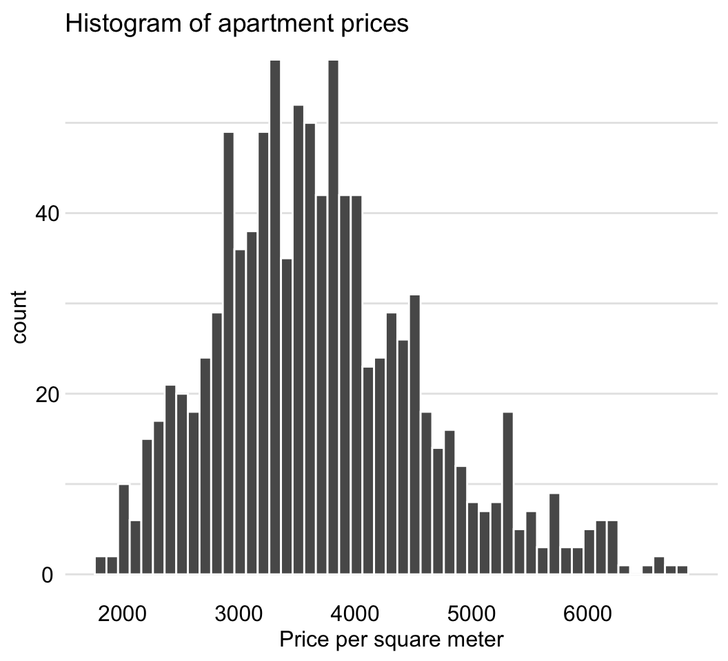
Figure 4.6: Distribution of the price per square meter in the apartment-prices data.
Figure 4.7 suggests (possibly) a non-linear relationship between construction.year and m2.price and a linear relation between surface and m2.price.
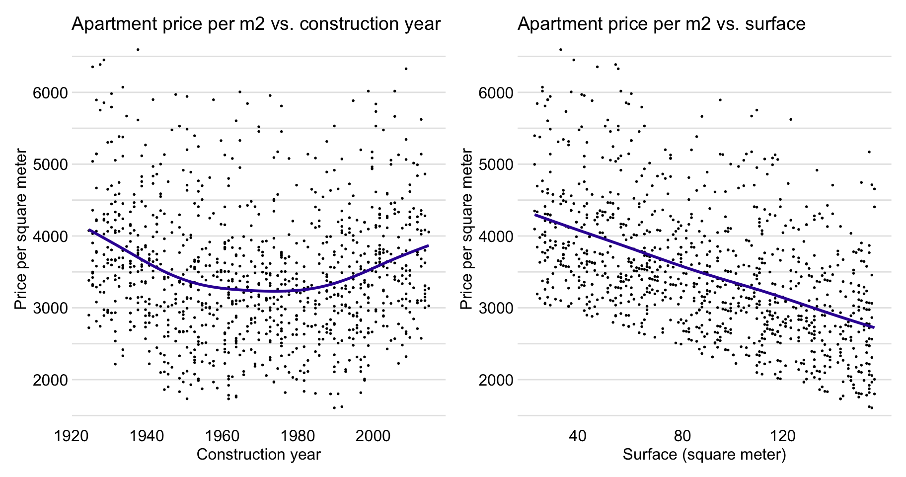
Figure 4.7: Apartment-prices data. Price per square meter vs. year of construction (left-hand-side panel) and vs. surface (right-hand-side panel).
Figure 4.8 indicates that the relationship between floor and m2.price is also close to linear, as well as is the association between no.rooms and m2.price .
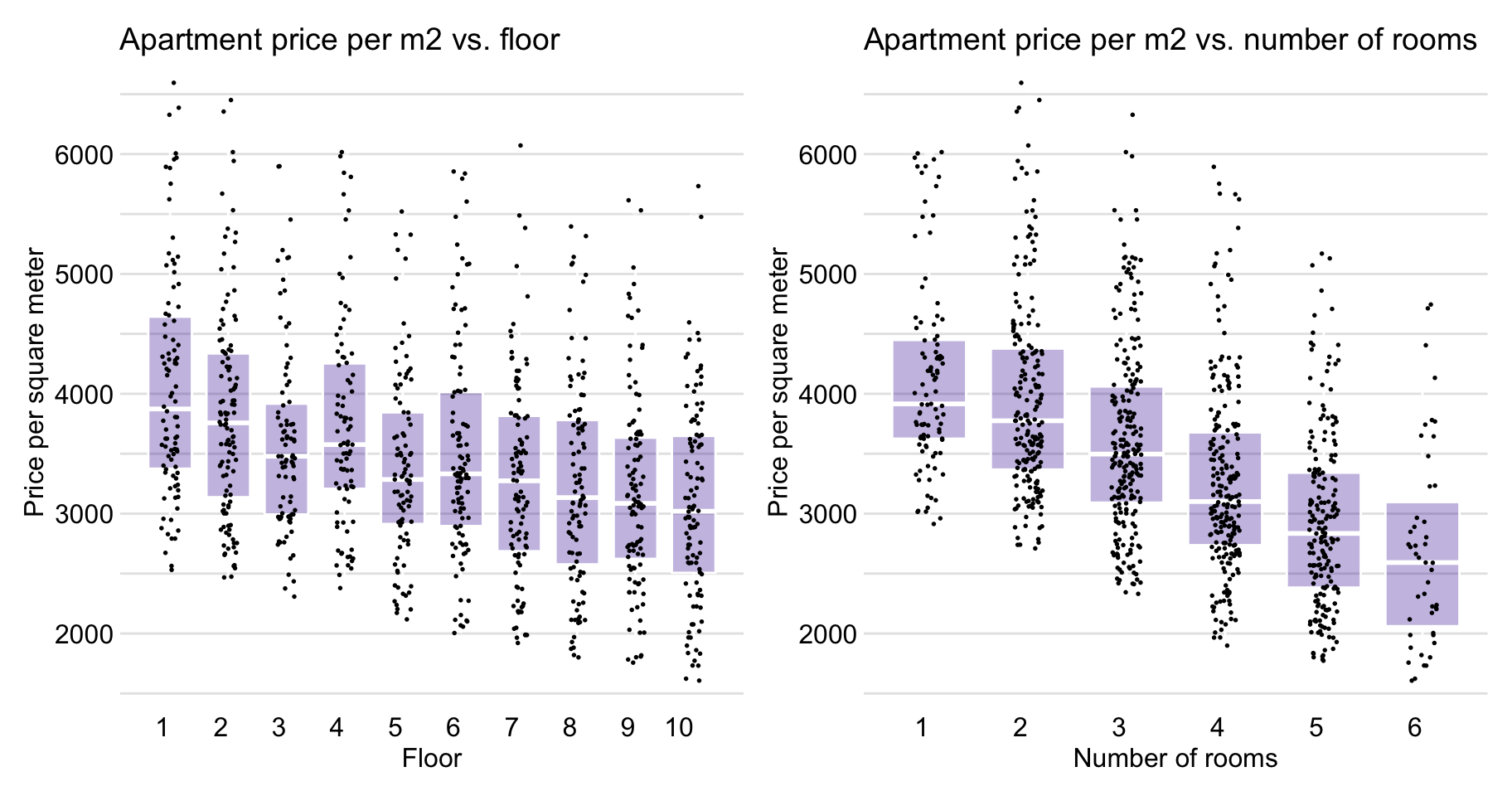
Figure 4.8: Apartment-prices data. Price per square meter vs. floor (left-hand-side panel) and vs. number of rooms (right-hand-side panel).
Figure 4.9 shows that surface and number of rooms are positively associated and that prices depend on the district. In particular, box plots in Figure 4.9 indicate that the highest prices per square meter are observed in Srodmiescie (Downtown).
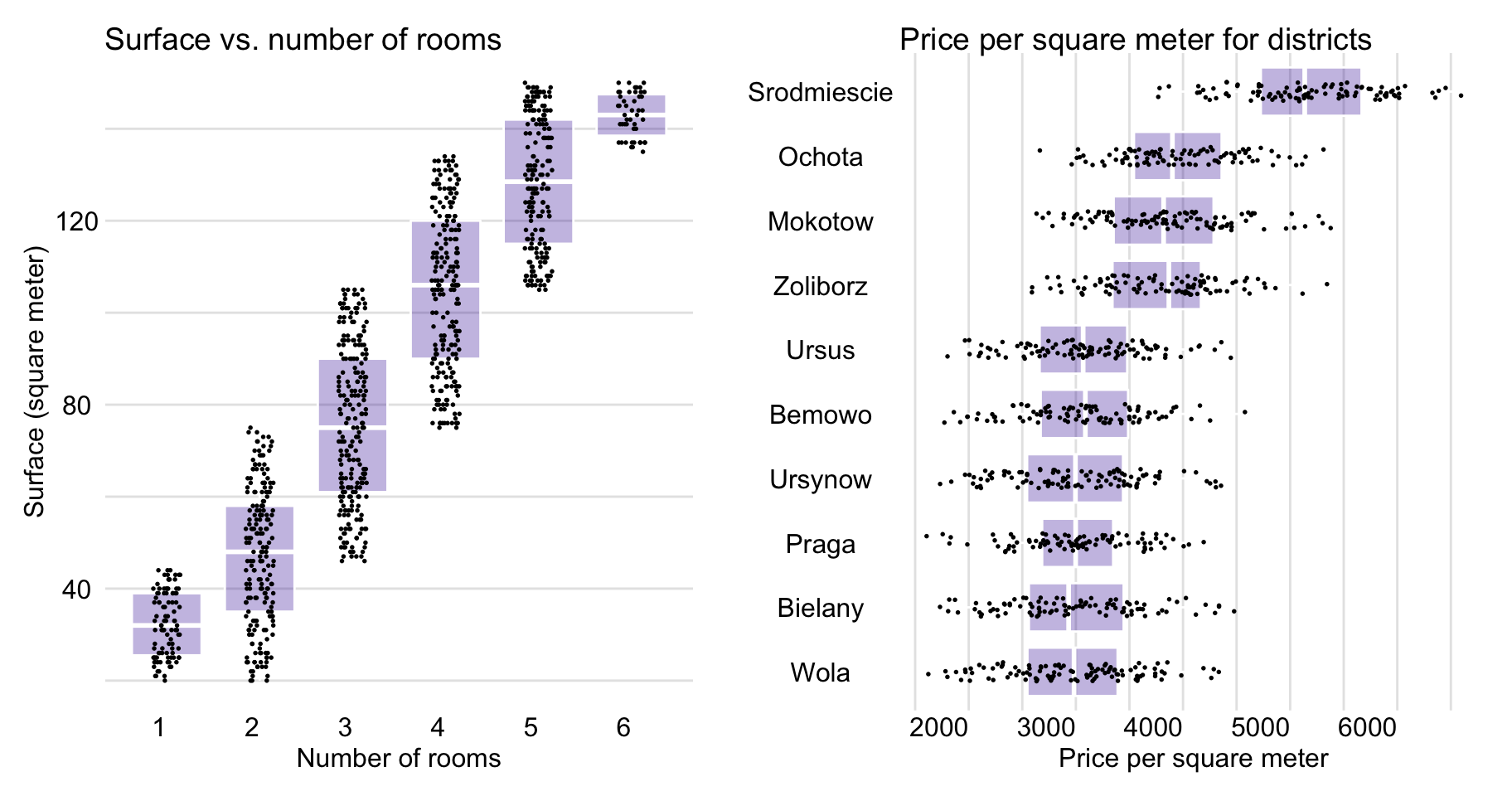
Figure 4.9: Apartment-prices data. Surface vs. number of rooms (left-hand-side panel) and price per square meter for different districts (right-hand-side panel).
4.5 Models for apartment prices, snippets for R
4.5.1 Linear regression model
The dependent variable of interest, m2.price, is continuous. Thus, a natural choice to build a predictive model is linear regression. We treat all the other variables in the apartments data frame as explanatory and include them in the model. To fit the model, we apply the lm() function. The results of the model are stored in model-object apartments_lm.
## Analysis of Variance Table
##
## Response: m2.price
##                    Df    Sum Sq   Mean Sq  F value    Pr(>F)
## construction.year   1   2629802   2629802   33.233 1.093e-08 ***
## surface             1 207840733 207840733 2626.541 < 2.2e-16 ***
## floor               1  79823027  79823027 1008.746 < 2.2e-16 ***
## no.rooms            1    956996    956996   12.094  0.000528 ***
## district            9 451993980  50221553  634.664 < 2.2e-16 ***
## Residuals         986  78023123     79131
## ---
## Signif. codes:  0 '***' 0.001 '**' 0.01 '*' 0.05 '.' 0.1 ' ' 1
4.5.2 Random forest model
As an alternative to linear regression, we consider a random forest model. Again, we treat all the variables in the apartments data frame other than m2.price as explanatory and include them in the model. To fit the model, we apply the randomForest() function, with default settings, from the package with the same name (Liaw and Wiener 2002). The results of the model are stored in model-object apartments_rf.
4.5.3 Support vector machine model
Finally, we consider an SVM model, with all the variables in the apartments data frame other than m2.price treated as explanatory. To fit the model, we use the svm() function, with default settings, from package e1071 (Meyer et al. 2019). The results of the model are stored in model-object apartments_svm.
4.5.4 Models’ predictions
The predict() function calculates predictions for a specific model. In the example below, we use model-objects apartments_lm, apartments_rf, and apartments_svm, to calculate predictions for prices of the apartments from the apartments_test data frame. Note that, for brevity’s sake, we compute the predictions only for the first six observations from the data frame.
The actual prices for the first six observations from apartments_test are provided below.
## [1] 4644 3082 2498 2735 2781 2936Predicted prices for the linear regression model are as follows:
##     1001     1002     1003     1004     1005     1006
## 4820.009 3292.678 2717.910 2922.751 2974.086 2527.043
Predicted prices for the random forest model take the following values:
##     1001     1002     1003     1004     1005     1006
## 4214.084 3178.061 2695.787 2744.775 2951.069 2999.450
Predicted prices for the SVM model are as follows:
##     1001     1002     1003     1004     1005     1006
## 4590.076 3012.044 2369.748 2712.456 2681.777 2750.904
By using the code presented below, we summarize the predictive performance of the linear regression and random forest models by computing the square root of the mean-squared-error (RMSE). For a “perfect” predictive model, which would predict all observations exactly, RMSE should be equal to 0. More information about RMSE can be found in Section 15.3.1.
predicted_apartments_lm <- predict(apartments_lm, apartments_test)
sqrt(mean((predicted_apartments_lm - apartments_test$m2.price)^2))
## [1] 283.0865predicted_apartments_rf <- predict(apartments_rf, apartments_test)
sqrt(mean((predicted_apartments_rf - apartments_test$m2.price)^2))## [1] 282.9519For the random forest model, RMSE is equal to 283. It is almost identical to the RMSE for the linear regression model, which is equal to 283.1. Thus, the question we may face is: should we choose the more complex but flexible random forest model, or the simpler and easier to interpret linear regression model? In the subsequent chapters, we will try to provide an answer to this question. In particular, we will show that a proper model exploration may help to discover weak and strong sides of any of the models and, in consequence, allow the creation of a new model, with better performance than either of the two.
4.5.5 Models’ explainers
The code presented below creates explainers for the models (see Sections 4.5.1–4.5.3) fitted to the apartment-prices data. Note that we use the apartments_test data frame without the first column, i.e., the m2.price variable, in the data argument. This will be the dataset to which the model will be applied (see Section 4.2.6). The m2.price variable is explicitly specified as the dependent variable in the y argument (see Section 4.2.6).
apartments_lm_exp <- explain(model = apartments_lm,
                             data = apartments_test[,-1],
                             y = apartments_test$m2.price,
                             label = "Linear Regression")
apartments_rf_exp <- explain(model = apartments_rf,
                             data = apartments_test[,-1],
                             y = apartments_test$m2.price,
                             label = "Random Forest")
apartments_svm_exp <- explain(model = apartments_svm,
                              data = apartments_test[,-1],
                              y = apartments_test$m2.price,
                              label = "Support Vector Machine")
4.5.6 List of model-objects
In Sections 4.5.1–4.5.3, we have built three predictive models for the apartments dataset. The models will be used in the rest of the book to illustrate the model-explanation methods and tools.
For the ease of reference, we summarize the models in Table 4.3. The binary model-objects can be downloaded by using the indicated archivist hooks (Biecek and Kosinski 2017). By calling a function specified in the last column of the table, one can restore a selected model in a local R environment.
| Model name / library | Link to this object |
|---|---|
apartments_lm |
Get the model: archivist:: |
stats:: lm v.3.5.3 |
aread("pbiecek/models/55f19"). |
apartments_rf |
Get the model: archivist:: |
randomForest:: randomForest v.4.6.14 |
aread("pbiecek/models/fe7a5"). |
apartments_svm |
Get the model: archivist:: |
e1071:: svm v.1.7.3 |
aread("pbiecek/models/d2ca0"). |
4.6 Models for apartment prices, snippets for Python
Apartment-prices data are provided in the apartments dataset, which is available in the dalex library. The values of the continuous dependent variable are given in the m2_price column; the remaining columns give the values of the explanatory variables that are used to construct the predictive models.
The following instructions load the apartments dataset and split it into the dependent variable y and the explanatory variables X.
import dalex as dx
apartments = dx.datasets.load_apartments()
X = apartments.drop(columns='m2_price')
y = apartments['m2_price']
Dataset X contains numeric variables with different ranges (for instance, surface and no.rooms) and categorical variables (district). Machine-learning algorithms in the sklearn library require data in a numeric form. Therefore, before modelling, we use a pipeline that performs data pre-processing. In particular, we scale the continuous variables (construction.year, surface, floor, and no.rooms) and one-hot-encode the categorical variables (district).
from sklearn.preprocessing import StandardScaler, OneHotEncoder
from sklearn.compose import make_column_transformer
from sklearn.pipeline import make_pipeline

preprocess = make_column_transformer(
    (StandardScaler(), ['construction_year', 'surface', 'floor', 'no_rooms']),
    (OneHotEncoder(), ['district']))
4.6.1 Linear regression model
To fit the linear regression model (see Section 4.5.1), we use the LinearRegression algorithm from the sklearn library. The fitted model is stored in object apartments_lm, which will be used in subsequent chapters.
4.6.2 Random forest model
To fit the random forest model (see Section 4.5.2), we use the RandomForestRegressor algorithm from the sklearn library. We apply the default settings with trees not deeper than three levels and the number of trees in the random forest set to 500. The fitted model is stored in object apartments_rf for purpose of illustrations in subsequent chapters.
4.6.3 Support vector machine model
Finally, to fit the SVM model (see Section 4.5.3), we use the SVR algorithm from the sklearn library. The fitted model is stored in object apartments_svm, which will be used in subsequent chapters.
4.6.4 Models’ predictions
Let us now compare predictions that are obtained from the different models for the apartments_test data. In the code below, we use the predict() method to obtain the predicted price per square meter for the linear regression model.
apartments_test = dx.datasets.load_apartments_test()
apartments_test = apartments_test.drop(columns='m2_price')

apartments_lm.predict(apartments_test)
# array([4820.00943156, 3292.67756996, 2717.90972101, ..., 4836.44370353,
#        3191.69063189, 5157.93680175])
In a similar way, we obtain the predictions for the two remaining models.
4.6.5 Models’ explainers
The Python-code examples presented for the models for the apartment-prices dataset use functions from the sklearn library, which facilitates uniform working with models. However, we may want to, or have to, work with models built by using other libraries. To simplify the task, the dalex library wraps models in objects of class Explainer that contain, in a uniform way, all the functions necessary for working with models (see Section 4.3.6). The code below creates explainer-objects for the models (see Sections 4.6.1–4.6.3) fitted to the apartment-prices data.
apartments_lm_exp = dx.Explainer(apartments_lm, X, y,
                      label = "Apartments LM Pipeline")
apartments_rf_exp = dx.Explainer(apartments_rf, X, y,
                      label = "Apartments RF Pipeline")
apartments_svm_exp = dx.Explainer(apartments_svm, X, y,
                      label = "Apartments SVM Pipeline")
When an explainer is created, the specified model and data are tested for consistency.
Diagnostic information is printed on the screen.
The following output shows diagnostic information for the apartments_lm model.
Preparation of a new explainer is initiated

  -> data              : 1000 rows 5 cols
  -> target variable   : Argument 'y' converted to a numpy.ndarray.
  -> target variable   : 1000 values
  -> model_class       : sklearn.pipeline.Pipeline (default)
  -> label             : Apartments LM Pipeline
  -> predict function  : <yhat at 0x117090840> will be used (default)
  -> predicted values  : min = 1.78e+03, mean = 3.49e+03, max = 6.18e+03
  -> residual function : difference between y and yhat (default)
  -> residuals         : min = -2.47e+02, mean = 2.06e-13, max = 4.69e+02
  -> model_info        : package sklearn

A new explainer has been created!
References
Biecek, Przemyslaw. 2018. “DALEX: Explainers for complex predictive models in R.” Journal of Machine Learning Research 19 (84): 1–5. http://jmlr.org/papers/v19/18-416.html.
Biecek, Przemyslaw, and Marcin Kosinski. 2017. “archivist: An R Package for Managing, Recording and Restoring Data Analysis Results.” Journal of Statistical Software 82 (11): 1–28. https://doi.org/10.18637/jss.v082.i11.
Breiman, Leo. 2001a. “Random Forests.” Machine Learning 45: 5–32. https://doi.org/10.1023/a:1010933404324.
Buuren, S. van. 2012. Flexible Imputation of Missing Data. Boca Raton, FL: Chapman; Hall/CRC.
Cortes, Corinna, and Vladimir Vapnik. 1995. “Support-Vector Networks.” Machine Learning, 273–97.
Friedman, Jerome H. 2000. “Greedy Function Approximation: A Gradient Boosting Machine.” Annals of Statistics 29: 1189–1232.
Harrell Jr, Frank E. 2018. Rms: Regression Modeling Strategies. https://CRAN.R-project.org/package=rms.
Liaw, Andy, and Matthew Wiener. 2002. “Classification and regression by randomForest.” R News 2 (3): 18–22. http://CRAN.R-project.org/doc/Rnews/.
Little, R. J. A., and D. B. Rubin. 2002. Statistical Analysis with Missing Data (2nd Ed.). Hoboken, NJ: Wiley.
Meyer, David, Evgenia Dimitriadou, Kurt Hornik, Andreas Weingessel, and Friedrich Leisch. 2019. E1071: Manual Functions of the Department of Statistics, Probability Theory Group (Formerly: E1071), Tu Wien. https://CRAN.R-project.org/package=e1071.
Molenberghs, G., and M. G. Kenward. 2007. Missing Data in Clinical Studies. Chichester, England: Wiley.
Ridgeway, Greg. 2017. Gbm: Generalized Boosted Regression Models. https://CRAN.R-project.org/package=gbm.
Schafer, J. L. 1997. Analysis of Incomplete Multivariate Data. Boca Raton, FL: Chapman; Hall/CRC.