11 Ceteris-paribus Oscillations
11.1 Introduction
Visual examination of ceteris-paribus (CP) profiles, as illustrated in the previous chapter, is insightful. However, in case of a model with a large number of explanatory variables, we may end up with a large number of plots that may be overwhelming. In such a situation, it might be useful to select the most interesting or important profiles. In this chapter, we describe a measure that can be used for such a purpose and that is directly linked to CP profiles. It can be seen as an instance-level variable-importance measure alternative to the measures discussed in Chapters 6–9.
11.2 Intuition
To assign importance to CP profiles, we can use the concept of profile oscillations. It is worth noting that the larger influence of an explanatory variable on prediction for a particular instance, the larger the fluctuations of the corresponding CP profile. For a variable that exercises little or no influence on a model’s prediction, the profile will be flat or will barely change. In other words, the values of the CP profile should be close to the value of the model’s prediction for a particular instance. Consequently, the sum of differences between the profile and the value of the prediction, taken across all possible values of the explanatory variable, should be close to zero. The sum can be graphically depicted by the area between the profile and the horizontal line representing the value of the single-instance prediction. On the other hand, for an explanatory variable with a large influence on the prediction, the area should be large. Figure 11.1 illustrates the concept based on CP profiles presented in Figure 10.4. The larger the highlighted area in Figure 11.1, the more important is the variable for the particular prediction.
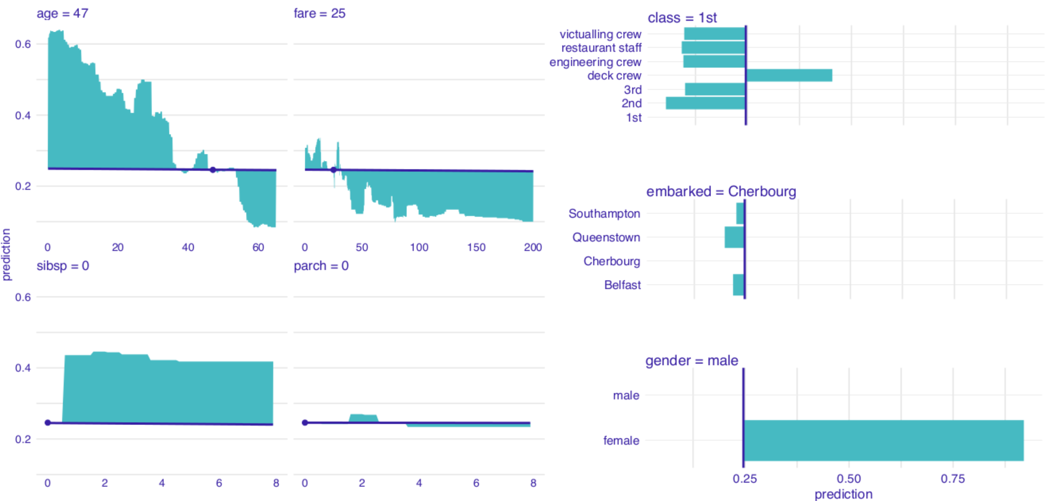
Figure 11.1: The value of the coloured area summarizes the oscillations of a ceteris-paribus (CP) profile and provides the mean of the absolute deviations between the CP profile and the single-instance prediction. The CP profiles are constructed for the titanic_rf random forest model for the Titanic data and passenger Henry.
11.3 Method
Let us formalize this concept now. Denote by \(g^j(z)\) the probability density function of the distribution of the \(j\)-th explanatory variable. The summary measure of the variable’s importance for model \(f()\)’s prediction at \(\underline{x}_*\), \(vip_{CP}^{j}(\underline{x}_*)\), is defined as follows:
\[\begin{equation} vip_{CP}^j(\underline{x}_*) = \int_{\mathcal R} |h^{j}_{\underline{x}_*}(z) - f(\underline{x}_*)| g^j(z)dz=E_{X^j}\left\{|h^{j}_{\underline{x}_*}(X^j) - f(\underline{x}_*)|\right\}. \tag{11.1} \end{equation}\]
Thus, \(vip_{CP}^j(\underline{x}_*)\) is the expected absolute deviation of the CP profile \(h^{j}_{\underline{x}_*}()\), defined in (10.1), from the model’s prediction at \(\underline{x}_*\), computed over the distribution \(g^j(z)\) of the \(j\)-th explanatory variable.
The true distribution of \(j\)-th explanatory variable is, in most cases, unknown. There are several possible approaches to construct an estimator of (11.1).
One is to calculate the area under the CP curve, i.e., to assume that \(g^j(z)\) is a uniform distribution over the range of variable \(X^j\). It follows that a straightforward estimator of \(vip_{CP}^{j}(\underline{x}_*)\) is
\[\begin{equation} \widehat{vip}_{CP}^{j,uni}(\underline{x}_*) = \frac 1k \sum_{l=1}^k |h^{j}_{x_*}(z_l) - f(\underline{x}_*)|, \tag{11.2} \end{equation}\]
where \(z_l\) (\(l=1, \ldots, k\)) are selected values of the \(j\)-th explanatory variable. For instance, one can consider all unique values of \(X^{j}\) in a dataset. Alternatively, for a continuous variable, one can use an equidistant grid of values.
Another approach is to use the empirical distribution of \(X^{j}\). This leads to the estimator defined as follows:
\[\begin{equation} \widehat{vip}_{CP}^{j,emp}(\underline{x}_*) = \frac 1n \sum_{i=1}^n |h^{j}_{\underline{x}_*}(x^{j}_i) - f(\underline{x}_*)|, \tag{11.3} \end{equation}\]
where index \(i\) runs through all observations in a dataset.
The use of \(\widehat{vip}_{CP}^{j,emp}(\underline{x}_*)\) is preferred when there are enough data to accurately estimate the empirical distribution and when the distribution is not uniform. On the other hand, \(\widehat{vip}_{CP}^{j,uni}(\underline{x}_*)\) is in most cases quicker to compute and, therefore, it is preferred if we look for fast approximations.
Note that the local evaluation of the variables’ importance can be very different from the global evaluation. This is well illustrated by the following example. Consider the model \[ f(x^1, x^2) = x^1 * x^2, \] where variables \(X^1\) and \(X^2\) take values in \([0,1]\). Furthermore, consider prediction for an observation described by vector \(\underline{x}_* = (0,1)\). In that case, the importance of \(X^1\) is larger than \(X^2\). This is because the CP profile \(h^1_{x_*}(z) = z\), while \(h^2_{x_*}(z) = 0\). Thus, there are oscillations for the first variable, but no oscillations for the second one. Hence, at \(\underline{x}_* = (0,1)\), the first variable is more important than the second. Globally, however, both variables are equally important, because the model is symmetrical.
11.4 Example: Titanic data
Figure 11.2 shows bar plots summarizing the size of oscillations for explanatory variables for the random forest model titanic_rf (see Section 4.2.2) for Henry, a 47-year-old man who travelled in the first class (see Section 4.2.5). The longer the bar, the larger the CP-profile oscillations for the particular explanatory variable. The left-hand-side panel presents the variable-importance measures computed by applying estimator \(\widehat{vip}_{CP}^{j,uni}(\underline{x}_*)\), given in (11.2), to an equidistant grid of values. The right-hand-side panel shows the results obtained by applying estimator \(\widehat{vip}_{CP}^{j,emp}(\underline{x}_*)\), given in (11.3), with an empirical distribution for explanatory variables.
The plots presented in Figure 11.2 indicate that both estimators consistently suggest that the most important variables for the model’s prediction for Henry are gender and age, followed by class. However, a remarkable difference can be observed for the sibsp variable, which gains in relative importance for estimator \(\widehat{vip}_{CP}^{j,uni}(\underline{x}_*)\). In this respect, it is worth recalling that this variable has a very skewed distribution (see Figure 4.3). In particular, a significant mass of the distribution is concentrated at zero, but there have been a few high values observed for the variable. As a result, the of empirical density is very different from a uniform distribution. Hence the difference in the relative importance noted in Figure 11.2.
It is worth noting that, while the variable-importance plot in Figure 11.2 does indicate which explanatory variables are important, it does not describe how do the variables influence the prediction. In that respect, the CP profile for age for Henry (see Figure 10.4) suggested that, if Henry were older, this would significantly lower his probability of survival. One the other hand, the CP profile for sibsp (see Figure 10.4) indicated that, were Henry not travelling alone, this would increase his chances of survival. Thus, the variable-importance plots should always be accompanied by plots of the relevant CP profiles.
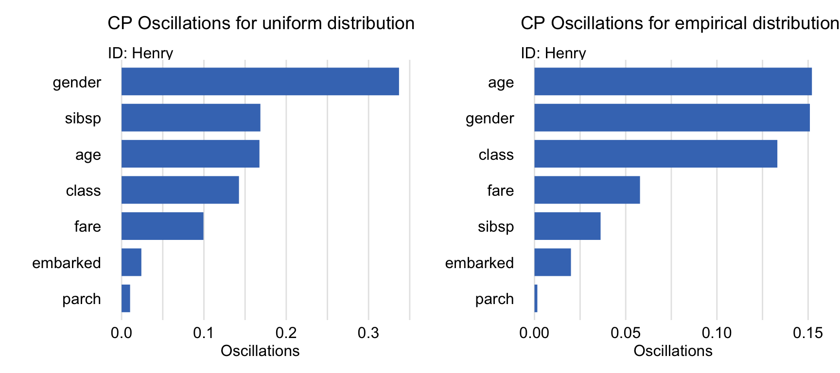
Figure 11.2: Variable-importance measures based on ceteris-paribus oscillations estimated by using (left-hand-side panel) a uniform grid of explanatory-variable values and (right-hand-side panel) empirical distribution of explanatory-variables for the random forest model and passenger Henry for the Titanic data.
11.5 Pros and cons
Oscillations of CP profiles are easy to interpret and understand. By using the average of oscillations, it is possible to select the most important variables for an instance prediction. This method can easily be extended to two or more variables.
There are several issues related to the use of the CP oscillations, though. For example, the oscillations may not be of help in situations when the use of CP profiles may itself be problematic (e.g., in the case of correlated explanatory variables or interactions – see Section 10.5). An important issue is that the CP-based variable-importance measures (11.1) do not fulfil the local accuracy condition (see Section 8.2), i.e., they do not sum up to the instance prediction for which they are calculated, unlike the break-down attributions (see Chapter 6) or Shapley values (see Chapter 8).
11.6 Code snippets for R
In this section, we present analysis of CP-profile oscillations as implemented in the DALEX package for R. For illustration, we use the random forest model titanic_rf (Section 4.2.2). The model was developed to predict the probability of survival after the sinking of the Titanic. Instance-level explanations are calculated for Henry, a 47-year-old male passenger that travelled in the first class (see Section 4.2.5).
We first retrieve the titanic_rf model-object and the data frame for Henry via the archivist hooks, as listed in Section 4.2.7. We also retrieve the version of the titanic data with imputed missing values.
titanic_imputed <- archivist::aread("pbiecek/models/27e5c")
titanic_rf <- archivist:: aread("pbiecek/models/4e0fc")
(henry <- archivist::aread("pbiecek/models/a6538"))
class gender age sibsp parch fare embarked
1 1st male 47 0 0 25 CherbourgThen we construct the explainer for the model by using the function explain() from the DALEX package (see Section 4.2.6). We also load the randomForest package, as the model was fitted by using function randomForest() from this package (see Section 4.2.2) and it is important to have the corresponding predict() function available. The model’s prediction for Henry is obtained with the help of that function.
library("randomForest")
library("DALEX")
explain_rf <- DALEX::explain(model = titanic_rf,
                          data = titanic_imputed[, -9],
                             y = titanic_imputed$survived == "yes",
                         label = "Random Forest")
predict(explain_rf, henry)
[1] 0.24611.6.1 Basic use of the predict_parts() function
To calculate CP-profile oscillations, we use the predict_parts() function, already introduced in Section 6.6. In particular, to use estimator \(\widehat{vip}_{CP}^{j,uni}(\underline{x}_*)\), defined in (11.2), we specify argument type="oscillations_uni", whereas for estimator \(\widehat{vip}_{CP}^{j,emp}(\underline{x}_*)\), defined in (11.3), we specify argument type="oscillations_emp". By default, oscillations are calculated for all explanatory variables. To perform calcualtions only for a subset of variables, one can use the variables argument.
In the code below, we apply the function to the explainer-object for the random forest model titanic_rf and the data frame for the instance of interest, i.e., henry. Additionally, we specify the type="oscillations_uni" argument to indicate that we want to compute CP-profile oscillations and the estimated value of the variable-importance measure as defined in (11.2).
oscillations_uniform <- predict_parts(explainer = explain_rf,
                                new_observation = henry,
                                           type = "oscillations_uni")
oscillations_uniform
## _vname_ _ids_ oscillations
## 2 gender 1 0.33700000
## 4 sibsp 1 0.16859406
## 3 age 1 0.16744554
## 1 class 1 0.14257143
## 6 fare 1 0.09942574
## 7 embarked 1 0.02400000
## 5 parch 1 0.01031683The resulting object is of class ceteris_paribus_oscillations, which is a data frame with three variables: _vname_, _ids_, and oscillations that provide, respectively, the name of the variable, the value of the identifier of the instance, and the estimated value of the variable-importance measure. Additionally, the object has also got an overloaded plot() function. We can use the latter function to plot the estimated values of the variable-importance measure for the instance of interest. In the code below, before creating the plot, we make the identifier for Henry more explicit. The resulting graph is shown in Figure 11.3.
oscillations_uniform$`_ids_` <- "Henry"
plot(oscillations_uniform) +
    ggtitle("Ceteris-paribus Oscillations",
"Expectation over uniform distribution (unique values)") 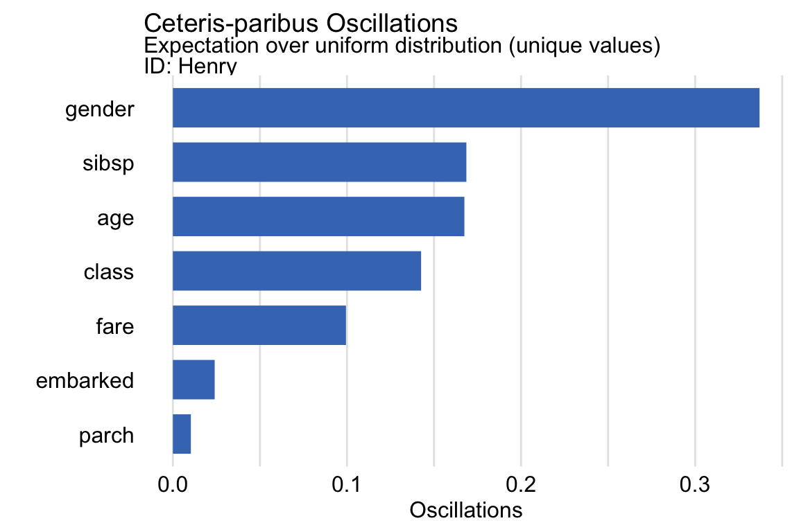
Figure 11.3: Variable-importance measures based on ceteris-paribus oscillations estimated by the oscillations_uni method of the predict_parts() function for the random forest model and passenger Henry for the Titanic data.
11.6.2 Advanced use of the predict_parts() function
As mentioned in the previous section, the predict_parts() function with argument type = "oscillations_uni" computes estimator \(\widehat{vip}_{CP}^{j,uni}(\underline{x}_*)\), defined in (11.2), while for argument type="oscillations_emp" it provides estimator \(\widehat{vip}_{CP}^{j,emp}(\underline{x}_*)\), defined in (11.3). However, one could also consider applying estimator \(\widehat{vip}_{CP}^{j,uni}(\underline{x}_*)\) but using a pre-defined grid of values for a continuous explanatory variable. Toward this aim, we can use the variable_splits argument to explicitly specify values for the density estimation. Its application is illustrated in the code below for variables age and fare. Note that, in this case, we use argument type = "oscillations". It is also worth noting that the use of the variable_splits argument limits the computations to the variables specified in the argument.
oscillations_equidist <- predict_parts(explain_rf, henry,
            variable_splits = list(age = seq(0, 65, 0.1),
                                  fare = seq(0, 200, 0.1),
                                gender = unique(titanic_imputed$gender),
                                 class = unique(titanic_imputed$class)),
                       type = "oscillations")
oscillations_equidist
## _vname_ _ids_ oscillations
## 3 gender 1 0.3370000
## 1 age 1 0.1677235
## 4 class 1 0.1425714
## 2 fare 1 0.1040790Subsequently, we can use the plot() function to construct a bar plot of the estimated values. In the code below, before creating the plot, we make the identifier for Henry more explicit. The resulting graph is shown in Figure 11.4.
oscillations_equidist$`_ids_` <- "Henry"
plot(oscillations_equidist) +
    ggtitle("Ceteris-paribus Oscillations",
            "Expectation over specified grid of points")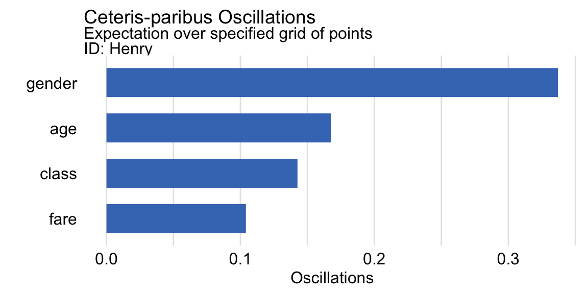
Figure 11.4: Variable-importance measures based on ceteris-paribus oscillations estimated by using a specified grid of points for the random forest model and passenger Henry for the Titanic data.
11.7 Code snippets for Python
At this point we are not aware about any Python libraries that would implement the methods presented in the current chapter.