21 FIFA 19
21.1 Introduction
In the previous chapters, we introduced a range of methods for the exploration of predictive models. Different methods were discussed in separate chapters, and while illustrated, they were not directly compared. Thus, in this chapter, we apply the methods to one dataset in order to present their relative merits. In particular, we present an example of a full process of a model development along the lines introduced in Chapter 2. This will allow us to show how one can combine results from different methods.
The Fédération Internationale de Football Association (FIFA) is a governing body of football (sometimes, especially in the USA, called soccer). FIFA is also a series of video games developed by EA Sports which faithfully reproduces the characteristics of real players. FIFA ratings of football players from the video game can be found at https://sofifa.com/. Data from this website for 2019 were scrapped and made available at the Kaggle webpage https://www.kaggle.com/karangadiya/fifa19.
We will use the data to build a predictive model for the evaluation of a player’s value. Subsequently, we will use the model exploration and explanation methods to better understand the model’s performance, as well as which variables and how to influence a player’s value.
21.2 Data preparation
The original dataset contains 89 variables that describe 16,924 players. The variables include information such as age, nationality, club, wage, etc. In what follows, we focus on 45 variables that are included in data frame fifa included in the DALEX package for R and Python. The variables from this dataset set are listed in Table 21.1.
| Name | Weak.Foot | FKAccuracy | Jumping | Composure |
| Club | Skill.Moves | LongPassing | Stamina | Marking |
| Position | Crossing | BallControl | Strength | StandingTackle |
| Value.EUR | Finishing | Acceleration | LongShots | SlidingTackle |
| Age | HeadingAccuracy | SprintSpeed | Aggression | GKDiving |
| Overall | ShortPassing | Agility | Interceptions | GKHandling |
| Special | Volleys | Reactions | Positioning | GKKicking |
| Preferred.Foot | Dribbling | Balance | Vision | GKPositioning |
| Reputation | Curve | ShotPower | Penalties | GKReflexes |
In particular, variable Value.EUR contains the player’s value in millions of EUR. This will be our dependent variable.
The distribution of the variable is heavily skewed to the right. In particular, the quartiles are equal to 325,000 EUR, 725,000 EUR, and 2,534,478 EUR. There are three players with a value higher than 100 millions of Euro.
Thus, in our analyses, we will consider a logarithmically-transformed players’ value. Figure 21.1 presents the empirical cumulative-distribution function and histogram for the transformed value. They indicate that the transformation makes the distribution less skewed.
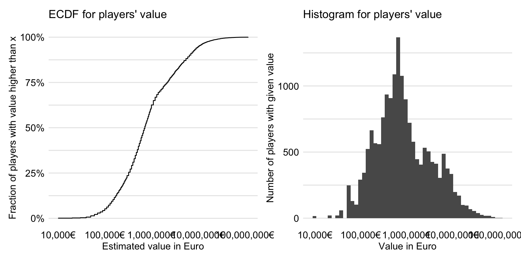
Figure 21.1: The empirical cumulative-distribution function and histogram for the log\(_{10}\)-transformed players’ values.
Additionally, we take a closer look at four characteristics that will be considered as explanatory variables later in this chapter. These are: Age, Reactions (a movement skill), BallControl (a general skill), and Dribbling (a general skill).
Figure 21.2 presents histograms of the values of the four variables. From the plot for Age we can conclude that most of the players are between 20 and 30 years of age (median age: 25). Variable Reactions has an approximately symmetric distribution, with quartiles equal to 56, 62, and 68. Histograms of BallControl and Dribbling indicate, interestingly, bimodal distributions. The smaller modes are due to goalkeepers.
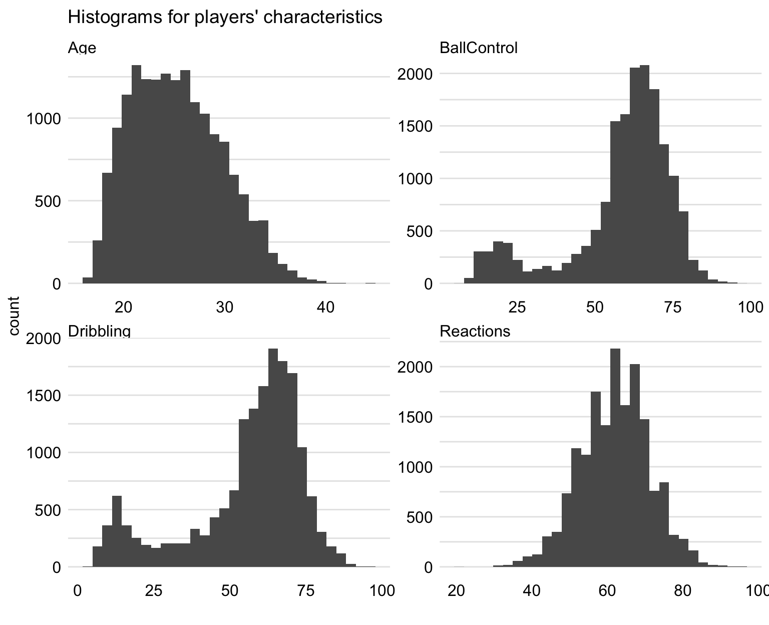
Figure 21.2: Histograms for selected characteristics of players.
21.2.1 Code snippets for R
The subset of 5000 most valuable players from the FIFA 19 data is available in the fifa data frame in the DALEX package.
21.3 Data understanding
We will investigate the relationship between the four selected characteristics and the (logarithmically-transformed) player’s value. Toward this aim, we use the scatter plots shown in Figure 21.3. Each plot includes a smoothed curve capturing the trend.
For Age, the relationship is not monotonic. There seems to be an optimal age, between 25 and 30 years, at which the player’s value reaches the maximum. On the other hand, the value of youngest and oldest players is about 10 times lower, as compared to the maximum.
For variables BallControl and Dribbling, the relationship is not monotonic. In general, the larger value of these coefficients, the large value of a player. However, there are “local” maxima for players with low scores for BallControl and Dribbling. As it was suggested earlier, these are probably goalkeepers.
For Reactions, the association with the player’s value is monotonic, with increasing values of the variable leading to increasing values of players.
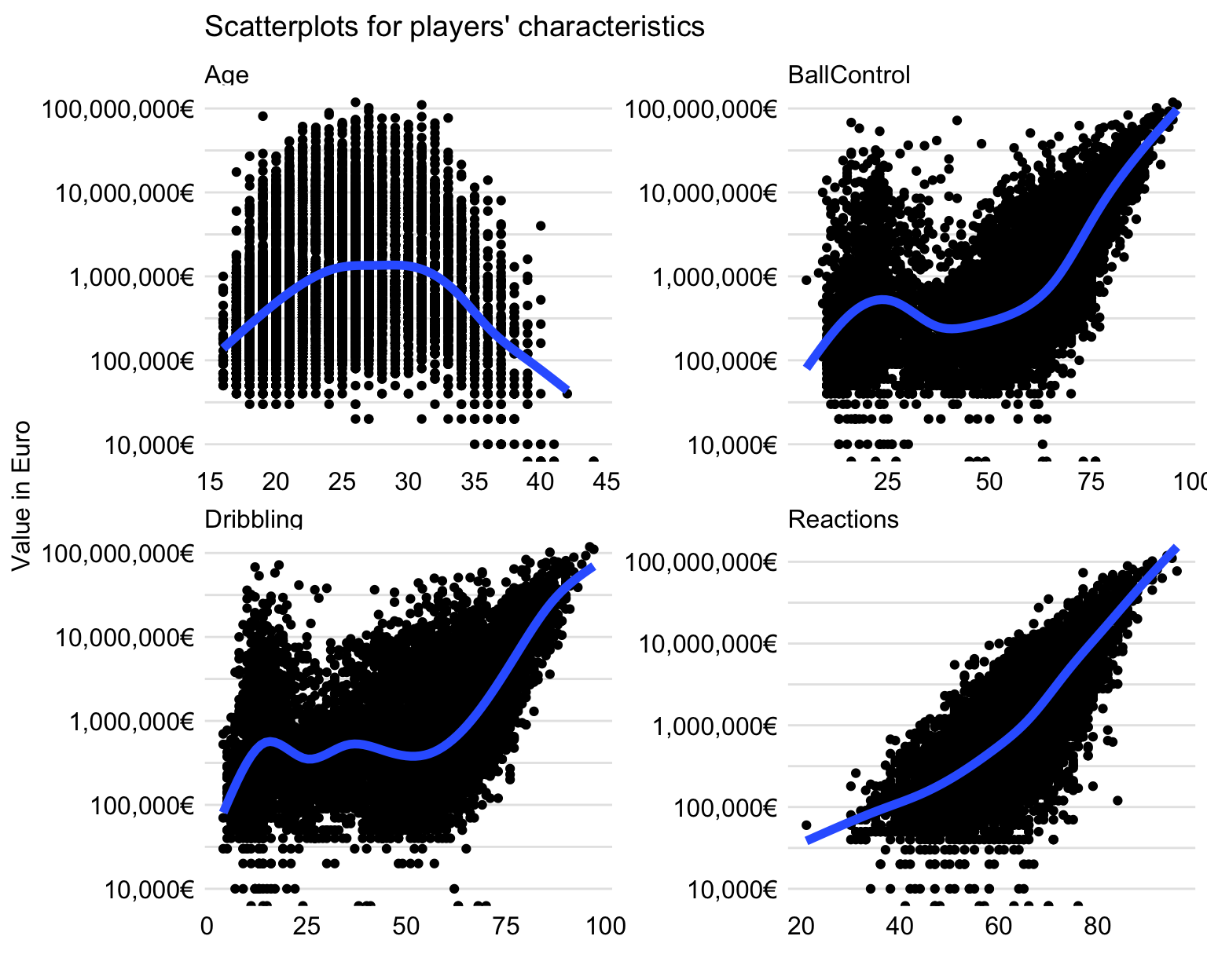
Figure 21.3: Scatter plots illustrating the relationship between the (logarithmically-transformed) player’s value and selected characteristics.
Figure 21.4 presents the scatter-plot matrix for the four selected variables. It indicates that all variables are positively correlated, though with different strength. In particular, BallControl and Dribbling are strongly correlated, with the estimated correlation coefficient larger than 0.9. Reactions is moderately correlated with the other three variables. Finally, there is a moderate correlation between Age and Reactions, but not much correlation with BallControl and Dribbling.
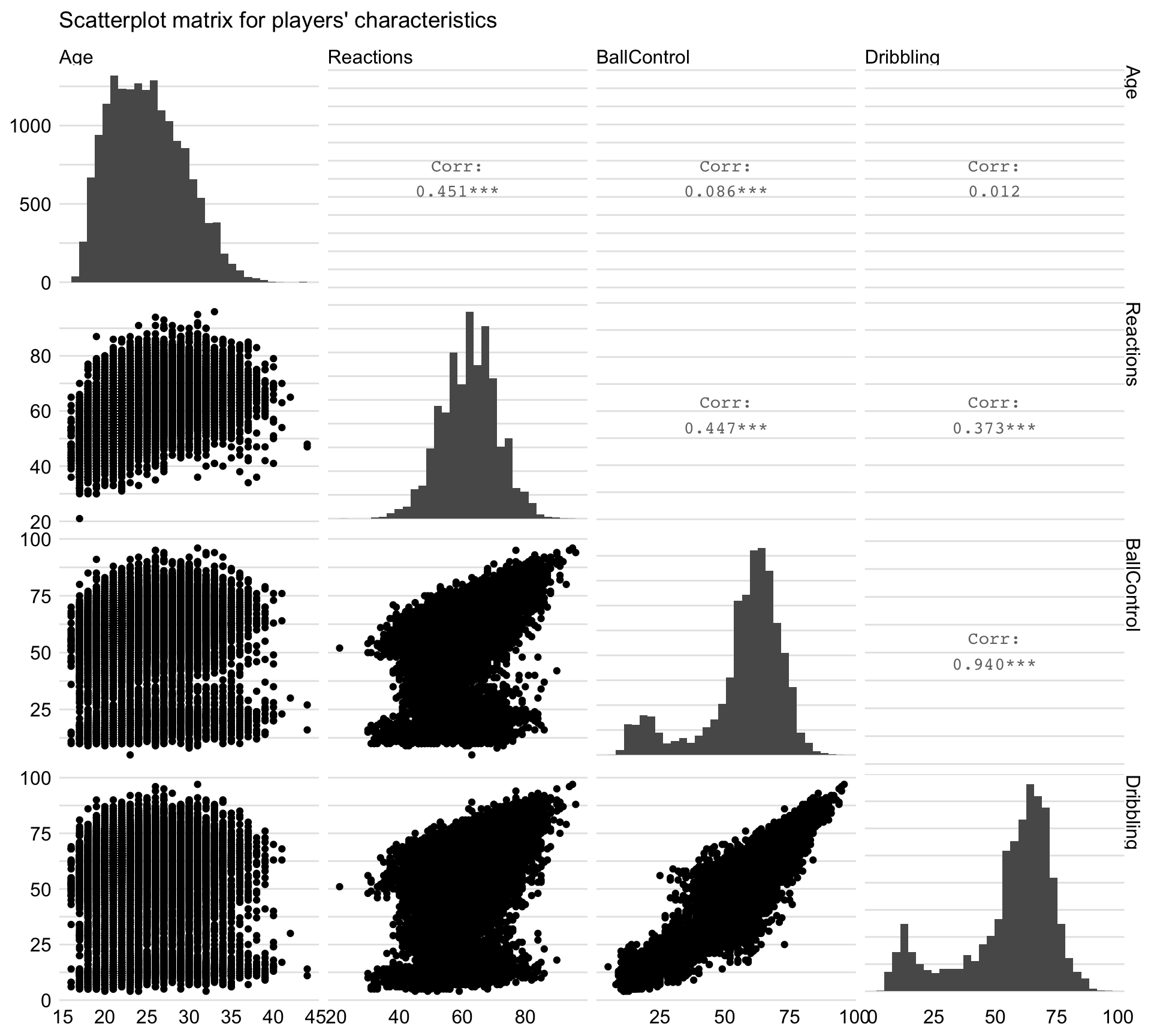
Figure 21.4: Scatter-plot matrix illustrating the relationship between selected characteristics of players.
21.4 Model assembly
In this section, we develop a model for players’ values. We consider all variables other than Name, Club, Position, Value.EUR, Overall, and Special (see Section 21.2) as explanatory variables. The base-10 logarithm of the player’s value is the dependent variable.
Given different possible forms of relationship between the (logarithmically-transformed) player’s value and explanatory variables (as seen, for example, in Figure 21.3), we build four different, flexible models to check whether they are capable of capturing the various relationships. In particular, we consider the following models:
- a boosting model with 250 trees of 1-level depth, as implemented in package
gbm(Ridgeway 2017), - a boosting model with 250 trees of 4-levels depth (this model should be able to catch interactions between variables),
- a random forest model with 250 trees, as implemented in package
ranger(Wright and Ziegler 2017), - a linear model with a spline-transformation of explanatory variables, as implemented in package
rms(Harrell Jr 2018).
These models will be explored in detail in the following sections.
21.4.1 Code snippets for R
In this section, we show R-code snippets used to develop the gradient boosting model. Other models were built in a similar way.
The code below fits the model to the data. The dependent variable LogValue contains the base-10 logarithm of Value.EUR, i.e., of the player’s value.
fifa$LogValue <- log10(fifa$Value.EUR)
fifa_small <- fifa[,-c(1, 2, 3, 4, 6, 7)]

fifa_gbm_deep <- gbm(LogValue~., data = fifa_small, n.trees = 250,
        interaction.depth = 4, distribution = "gaussian")
For model-exploration purposes, we have got to create an explainer-object with the help of the DALEX::explain() function (see Section 4.2.6). The code below is used for the gradient boosting model. Note that the model was fitted to the logarithmically-transformed player’s value. However, it is more natural to interpret the predictions on the original scale. This is why, in the provided syntax, we apply the predict_function argument to specify a user-defined function to obtain predictions on the original scale, in Euro. Additionally, we use the data and y arguments to indicate the data frame with explanatory variables and the values of the dependent variable, for which predictions are to be obtained. Finally, the model receives its own label.
21.4.2 Code snippets for Python
In this section, we show Python-code snippets used to develop the gradient boosting model. Other models were built in a similar way.
The code below fits the model to the data. The dependent variable ylog contains the logarithm of value_eur, i.e., of the player’s value.
from lightgbm import LGBMRegressor
from sklearn.model_selection import train_test_split
import numpy as np

X = fifa.drop(["nationality", "overall", "potential",
     "value_eur", "wage_eur"], axis = 1)
y = fifa['value_eur']
ylog = np.log(y)

X_train, X_test, ylog_train, ylog_test, y_train, y_test =
     train_test_split(X, ylog, y, test_size = 0.25, random_state = 4)
gbm_model = LGBMRegressor()
gbm_model.fit(X_train, ylog_train, verbose = False)
For model-exploration purposes, we have to create the explainer-object with the help of the Explainer() constructor from the dalex library (see Section 4.3.6). The code is provided below. Note that the model was fitted to the logarithmically-transformed player’s value. However, it is more natural to interpret the predictions on the original scale. This is why, in the provided syntax, we apply the predict_function argument to specify a user-defined function to obtain predictions on the original scale, in Euro. Additionally, we use the X and y arguments to indicate the data frame with explanatory variables and the values of the dependent variable, for which predictions are to be obtained. Finally, the model receives its own label.
21.5 Model audit
Having developed the four candidate models, we may want to evaluate their performance. Toward this aim, we can use the measures discussed in Section 15.3.1. The computed values are presented in Table 21.2. On average, the values of the root-mean-squared-error (RMSE) and mean-absolute-deviation (MAD) are the smallest for the random forest model.
| MSE | RMSE | R2 | MAD | |
|---|---|---|---|---|
| GBM shallow | 8.990694e+12 | 2998449 | 0.7300429 | 183682.91 |
| GBM deep | 2.211439e+12 | 1487091 | 0.9335987 | 118425.56 |
| RF | 1.141176e+12 | 1068258 | 0.9657347 | 50693.24 |
| RM | 2.191297e+13 | 4681129 | 0.3420350 | 148187.06 |
In addition to computing measures of the overall performance of the model, we should conduct a more detailed examination of both overall- and instance-specific performance. Toward this aim, we can apply residual diagnostics, as discussed in Chapter 19.
For instance, we can create a plot comparing the predicted (fitted) and observed values of the dependent variable.
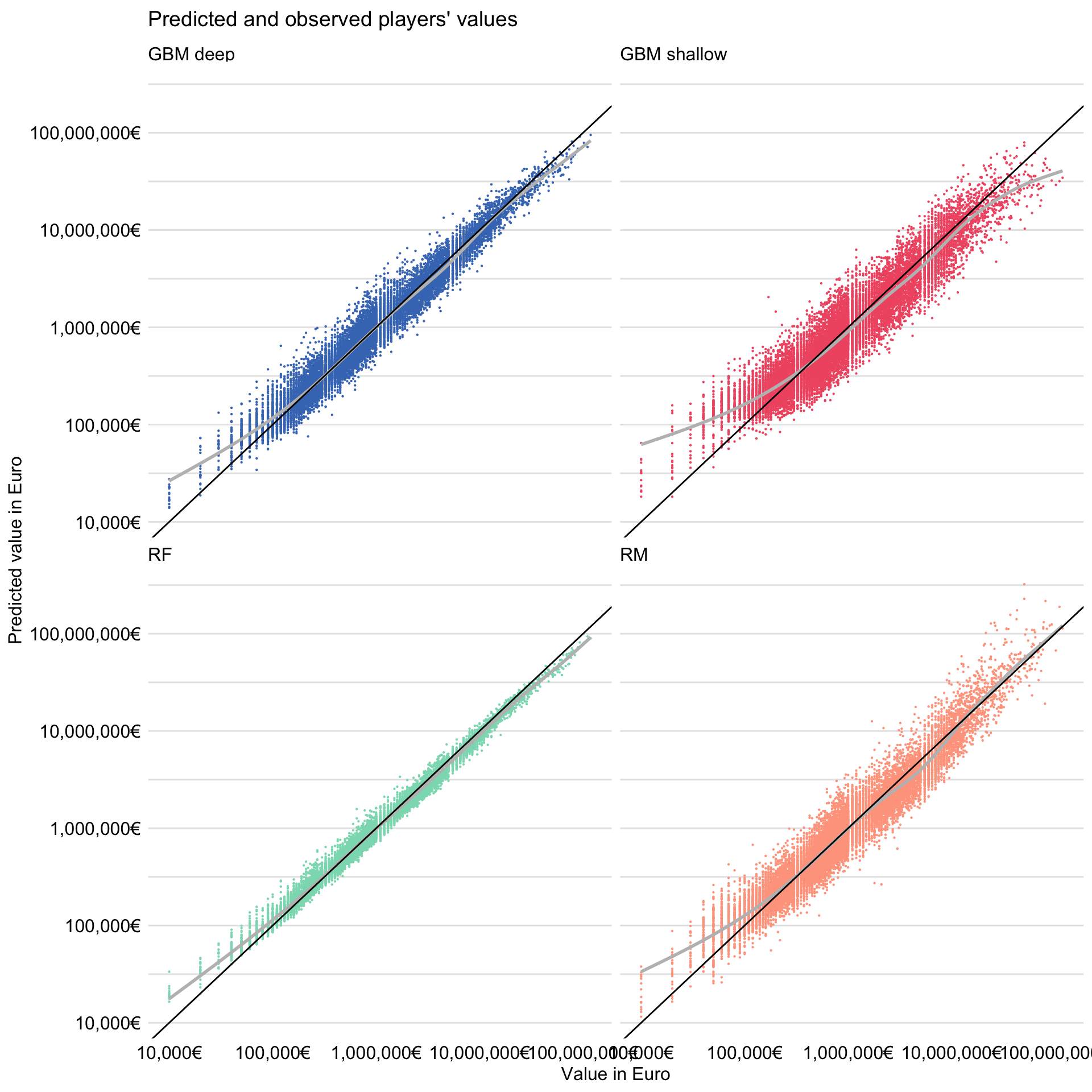
Figure 21.5: Observed and predicted (fitted) players’ values for the four models for the FIFA 19 data.
The resulting plot is shown in Figure 21.5. It indicates that predictions are closest to the observed values of the dependent variable for the random forest model. It is worth noting that the smoothed trend for the model is close to a straight line, but with a slope smaller than 1. This implies the random forest model underestimates the actual value of the most expensive players, while it overestimates the value for the least expensive ones. A similar pattern can be observed for the gradient boosting models. This “shrinking to the mean” is typical for this type of models.
21.5.1 Code snippets for R
In this section, we show R-code snippets for model audit for the gradient boosting model. For other models a similar syntax was used.
The model_performance() function (see Section 15.6) is used to calculate the values of RMSE, MSE, R\(^2\), and MAD for the model.
The model_diagnostics() function (see Section 19.6) is used to create residual-diagnostics plots. Results of this function can be visualised with the generic plot() function. In the code that follows, additional arguments are used to improve the outlook and interpretability of both axes.
fifa_md_gbm_deep <- model_diagnostics(fifa_gbm_exp_deep)
plot(fifa_md_gbm_deep,
     variable = "y", yvariable = "y_hat") +
  scale_x_continuous("Value in Euro", trans = "log10",
                      labels = dollar_format(suffix = "€", prefix = "")) +
  scale_y_continuous("Predicted value in Euro", trans = "log10",
                     labels = dollar_format(suffix = "€", prefix = "")) +
  geom_abline(slope = 1) +
  ggtitle("Predicted and observed players' values", "")
21.5.2 Code snippets for Python
In this section, we show Python-code snippets used to perform residual diagnostic for trained the gradient boosting model. Other models were tested in a similar way.
The fifa_gbm_exp.model_diagnostics() function (see Section 19.7) is used to calculate the residuals and absolute residuals.
Results of this function can be visualised with the plot() function. The code below produce diagnostic plots similar to these presented in Figure 21.5.
21.6 Model understanding (dataset-level explanations)
All four developed models involve many explanatory variables. It is of interest to understand which of the variables exercises the largest influence of models’ predictions. Toward this aim, we can apply the permutation-based variable-importance measure discussed in Chapter 16. Subsequently, we can construct a plot of the obtained mean (over the default 10 permutations) variable-importance measures. Note that we consider only the top-20 variables.
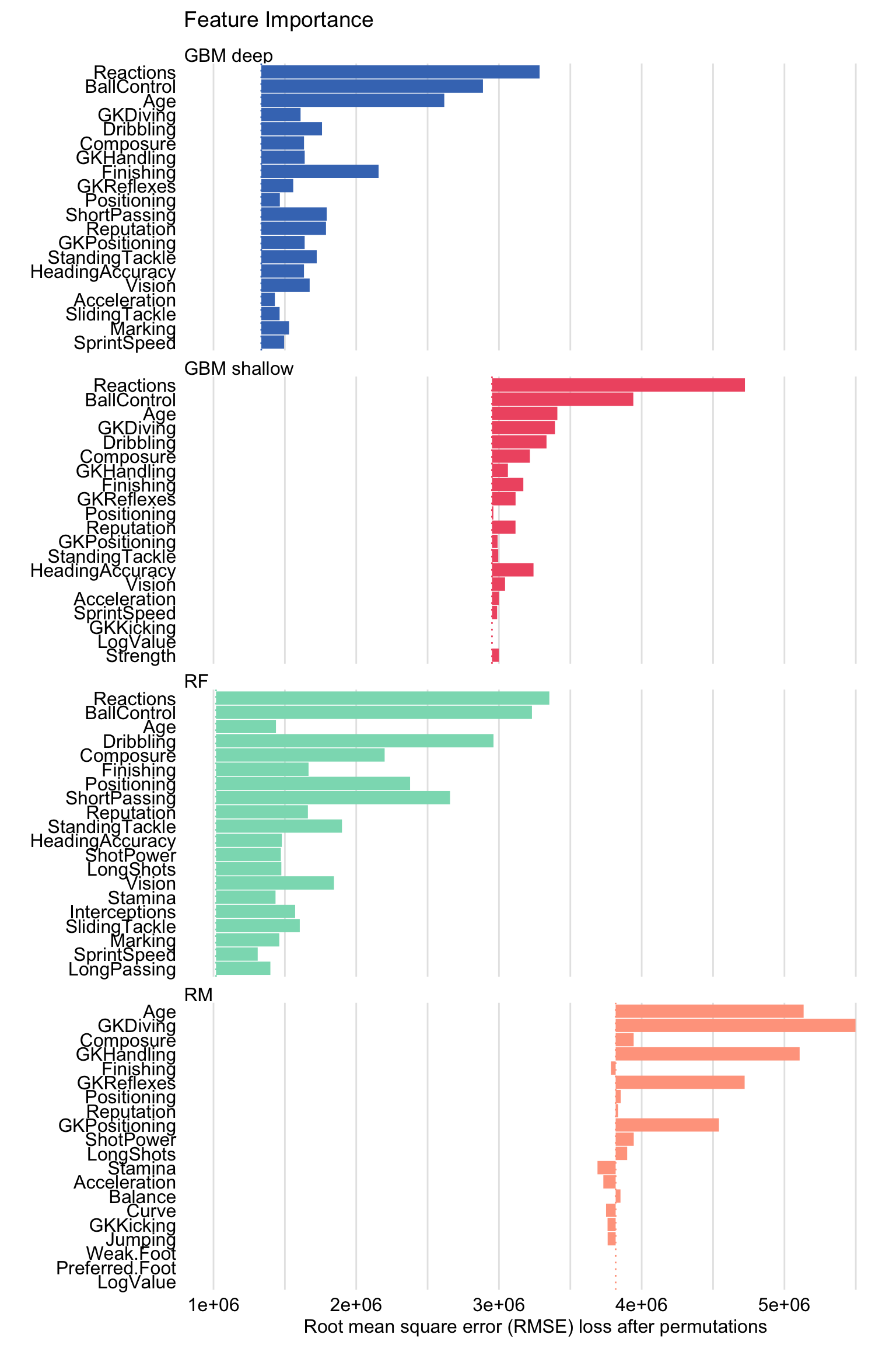
Figure 21.6: Mean variable-importance calculated using 10 permutations for the four models for the FIFA 19 data.
The resulting plot is shown in Figure 21.6. The bar for each explanatory variable starts at the RMSE value of a particular model and ends at the (mean) RMSE calculated for data with permuted values of the variable.
Figure 21.6 indicates that, for the gradient boosting and random forest models, the two explanatory variables with the largest values of the importance measure are Reactions or BallControl. The importance of other variables varies depending on the model. Interestingly, in the linear-regression model, the highest importance is given to goal-keeping skills.
We may also want to take a look at the partial-dependence (PD) profiles discussed in Chapter 17. Recall that they illustrate how does the expected value of a model’s predictions behave as a function of an explanatory variable. To create the profiles, we apply function model_profile() from the DALEX package (see Section 17.6). We focus on variables Reactions, BallControl, and Dribbling that were important in the random forest model (see Figure 21.6). We also consider Age, as it had some effect in the gradient boosting models. Subsequently, we can construct a plot of contrastive PD profiles (see Section 17.3.4) that is shown in Figure 21.7.
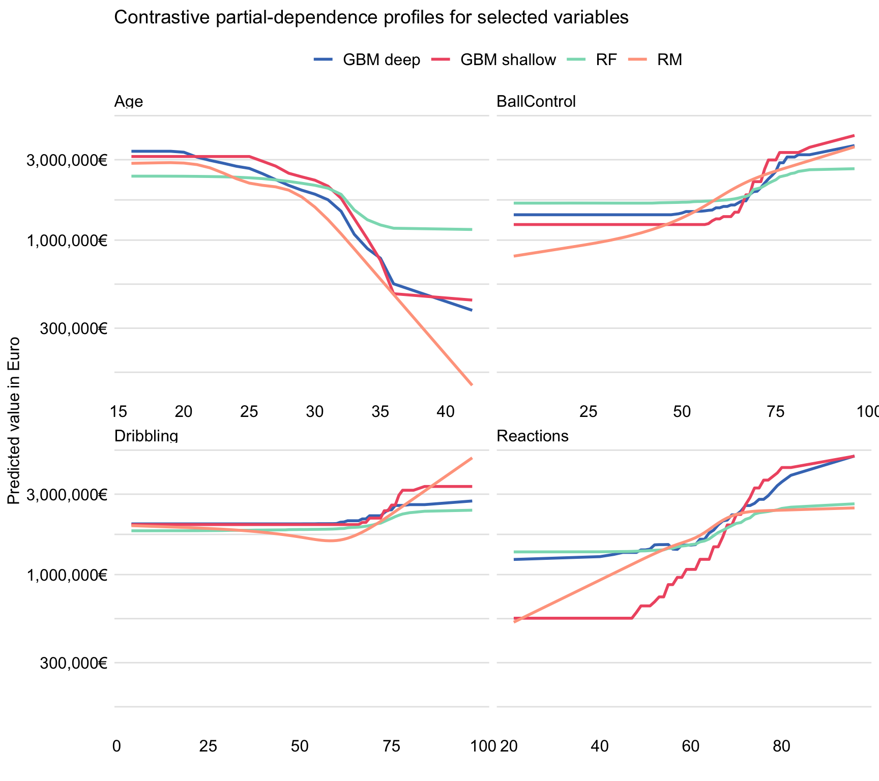
Figure 21.7: Contrastive partial-dependence profiles for the four models and selected explanatory variables for the FIFA 19 data.
Figure 21.7 indicates that the shape of the PD profiles for Reactions, BallControl, and Dribbling is, in general, similar for all the models and implies an increasing predicted player’s value for an increasing (at least, after passing some threshold) value of the explanatory variable. However, for Age, the shape is different and suggests a decreasing player’s value after the age of about 25 years. It is worth noting that the range of expected model’s predictions is, in general, the smallest for the random forest model. Also, the three tree-based models tend to stabilize the predictions at the ends of the explanatory-variable ranges.
The most interesting difference between the conclusions drawn from Figure 21.3 and those obtained from Figure 21.7 is observed for variable Age. In particular, Figure 21.3 suggests that the relationship between player’s age and value is non-monotonic, while Figure 21.7 suggests a non-increasing relationship. How can we explain this difference? A possible explanation is as follows. The youngest players have lower values, not because of their age, but because of their lower skills, which are correlated (as seen from the scatter-plot matrix in Figure 21.4) with young age. The simple data exploration analysis, presented in the upper-left panel of Figure 21.3, cannot separate the effects of age and skills. As a result, the analysis suggests a decrease in player’s value for the youngest players. In models, however, the effect of age is estimated while adjusting for the effect of skills. After this adjustment, the effect takes the form of a non-increasing pattern, as shown by the PD profiles for Age in Figure 21.7.
This example indicates that exploration of models may provide more insight than exploration of raw data. In exploratory data analysis, the effect of variable Age was confounded by the effect of skill-related variables. By using a model, the confounding has been removed.
21.6.1 Code snippets for R
In this section, we show R-code snippets for dataset-level exploration for the gradient boosting model. For other models a similar syntax was used.
The model_parts() function from the DALEX package (see Section 16.6) is used to calculate the permutation-based variable-importance measure. The generic plot() function is applied to graphically present the computed values of the measure. The max_vars argument is used to limit the number of presented variables up to 20.
fifa_mp_gbm_deep <- model_parts(fifa_gbm_exp_deep)
plot(fifa_mp_gbm_deep, max_vars = 20,
     bar_width = 4, show_boxplots = FALSE)
The model_profile() function from the DALEX package (see Section 17.6) is used to calculate PD profiles. The generic plot() function is used to graphically present the profiles for selected variables.
21.6.2 Code snippets for Python
In this section, we show Python code snippets for dataset-level exploration for the gradient boosting model. For other models a similar syntax was used.
The model_parts() method from the dalex library (see Section 16.7) is used to calculate the permutation-based variable-importance measure. The plot() method is applied to graphically present the computed values of the measure.
The model_profile() method from the dalex library (see Section 17.7) is used to calculate PD profiles. The plot() method is used to graphically present the computed profiles.
fifa_mp_gbm = fifa_gbm_exp.model_profile()

fifa_mp_gbm.plot(variables = ['movement_reactions',
    'skill_ball_control', 'skill_dribbling', 'age'])
In order to calculated other types of profiles, just change the type argument.
21.7 Instance-level explanations
After evaluation of the models at the dataset-level, we may want to focus on particular instances.
21.7.1 Robert Lewandowski
As a first example, we take a look at the value of Robert Lewandowski, for an obvious reason. Table 21.3 presents his characteristics, as included in the analyzed dataset. Robert Lewandowski is a striker.
| variable | value | variable | value | variable | value | variable | value |
|---|---|---|---|---|---|---|---|
| Age | 29 | Dribbling | 85 | ShotPower | 88 | Composure | 86 |
| Preferred.Foot | 2 | Curve | 77 | Jumping | 84 | Marking | 34 |
| Reputation | 4 | FKAccuracy | 86 | Stamina | 78 | StandingTackle | 42 |
| Weak.Foot | 4 | LongPassing | 65 | Strength | 84 | SlidingTackle | 19 |
| Skill.Moves | 4 | BallControl | 89 | LongShots | 84 | GKDiving | 15 |
| Crossing | 62 | Acceleration | 77 | Aggression | 80 | GKHandling | 6 |
| Finishing | 91 | SprintSpeed | 78 | Interceptions | 39 | GKKicking | 12 |
| HeadingAccuracy | 85 | Agility | 78 | Positioning | 91 | GKPositioning | 8 |
| ShortPassing | 83 | Reactions | 90 | Vision | 77 | GKReflexes | 10 |
| Volleys | 89 | Balance | 78 | Penalties | 88 | LogValue | 8 |
First, we take a look at variable attributions, discussed in Chapter 6. Recall that they decompose model’s prediction into parts that can be attributed to different explanatory variables. The attributions can be presented in a break-down (BD) plot. For brevity, we only consider the random forest model. The resulting BD plot is shown in Figure 21.8.
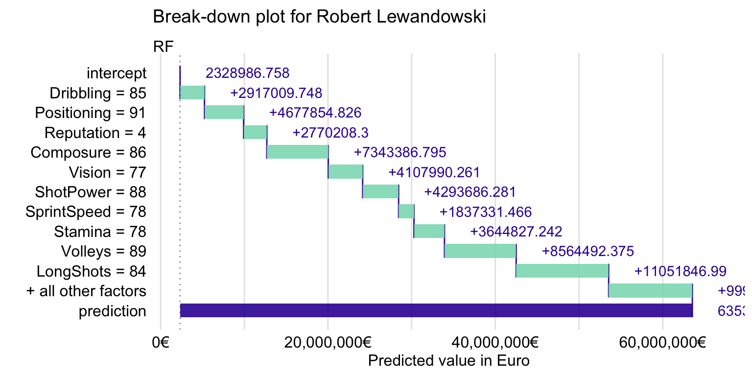
Figure 21.8: Break-down plot for Robert Lewandowski for the random forest model.
Figure 21.8 suggests that the explanatory variables with the largest effect are Composure, Volleys, LongShots, and Stamina. However, in Chapter 6 it was mentioned that variable attributions may depend on the order of explanatory covariates that are used in calculations. Thus, in Chapter 8 we introduced Shapley values, based on the idea of averaging the attributions over many orderings. Figure 21.9 presents the means of the Shapley values computed by using 25 random orderings for the random forest model.
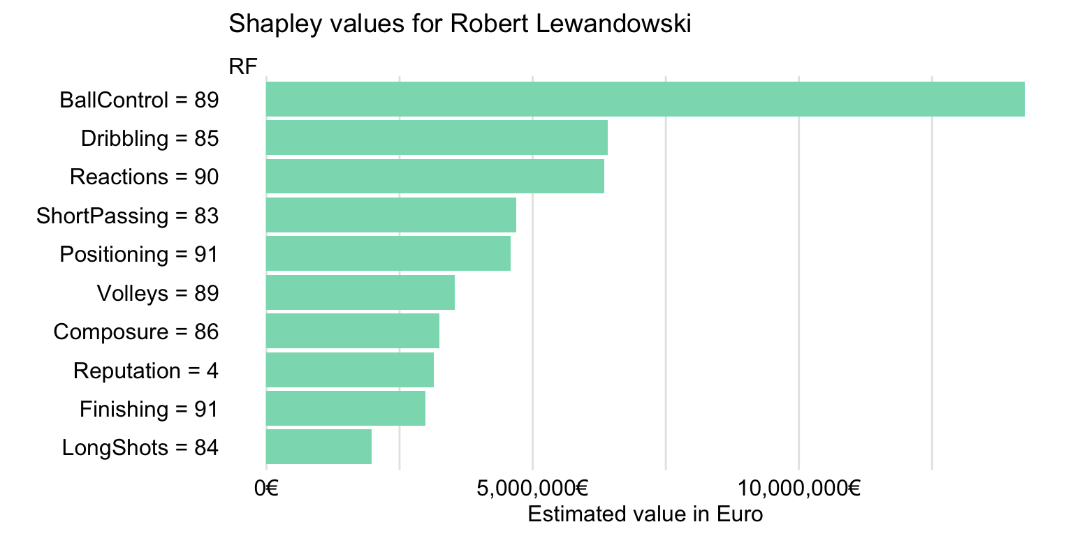
Figure 21.9: Shapley values for Robert Lewandowski for the random forest model.
Figure 21.9 indicates that the five explanatory variables with the largest Shapley values are BallControl, Dribbling, Reactions, ShortPassing, and Positioning. This makes sense, as Robert Lewandowski is a striker.
In Chapter 10, we introduced ceteris-paribus (CP) profiles. They capture the effect of a selected explanatory variable in terms of changes in a model’s prediction induced by changes in the variable’s values. Figure 21.10 presents the profiles for variables Age, Reactions, BallControl, and Dribbling for the random forest model.
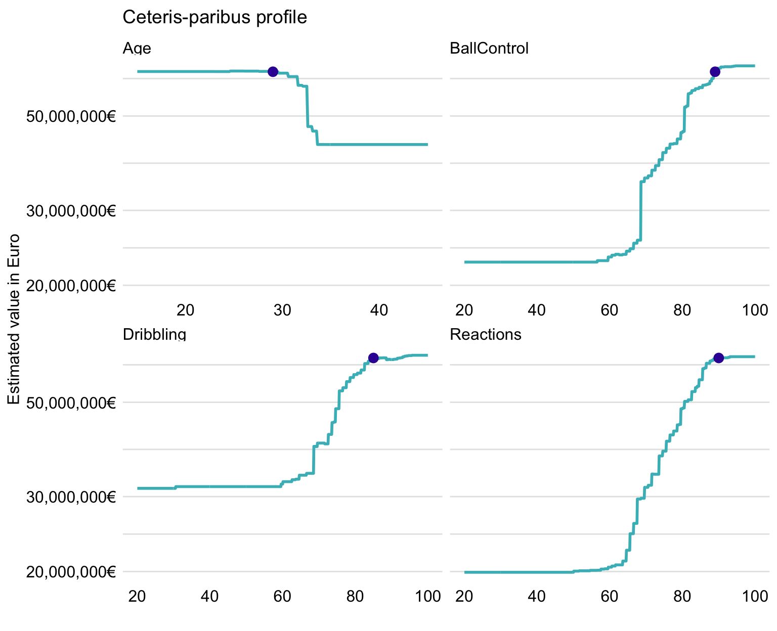
Figure 21.10: Ceteris-paribus profiles for Robert Lewandowski for four selected variables and the random forest model.
Figure 21.10 suggests that, among the four variables, BallControl and Reactions lead to the largest changes of predictions for this instance. For all four variables, the profiles flatten at the left- and right-hand-side edges. The predicted value of Robert Lewandowski reaches or is very close to the maximum for all four profiles. It is interesting to note that, for Age, the predicted value is located at the border of the age region at which the profile suggests a sharp drop in player’s value.
As it was argued in Chapter 12, it is worthwhile to check how does the model behave for observations similar to the instance of interest. Towards this aim, we may want to compare the distribution of residuals for “neighbors” of Robert Lewandowski. Figure 21.11 presents the histogram of residuals for all data and the 30 neighbors of Robert Lewandowski.
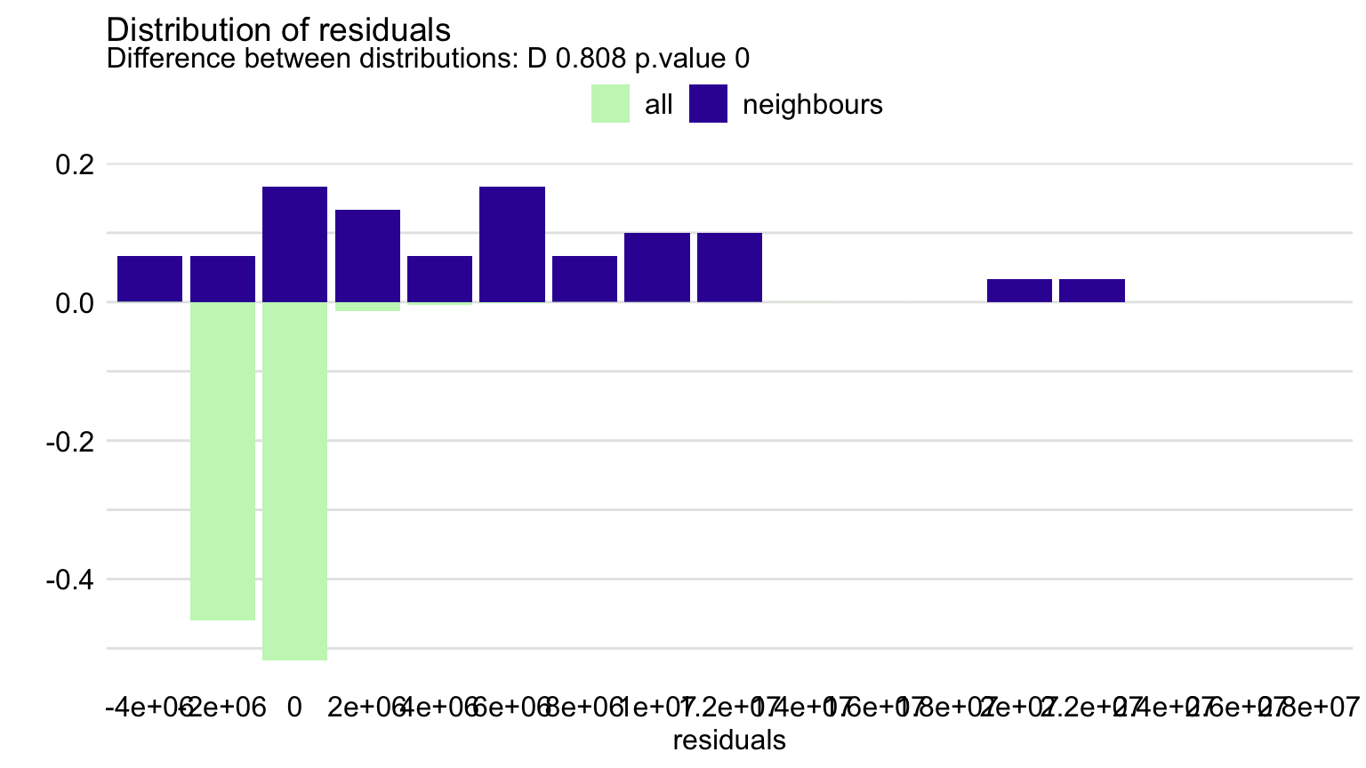
Figure 21.11: Distribution of residuals for the random forest model for all players and for 30 neighbors of Robert Lewandowski.
Clearly, the neighbors of Robert Lewandowski include some of the most expensive players. Therefore, as compared to the overall distribution, the distribution of residuals for the neighbors, presented in Figure 21.11, is skewed to the right, and its mean is larger than the overall mean. Thus, the model underestimates the actual value of the most expensive players. This was also noted based on the plot in the bottom-left panel of Figure 21.5.
We can also look at the local-stability plot, i.e., the plot that includes CP profiles for the nearest neighbors and the corresponding residuals (see Chapter 12). In Figure 21.12, we present the plot for Age.
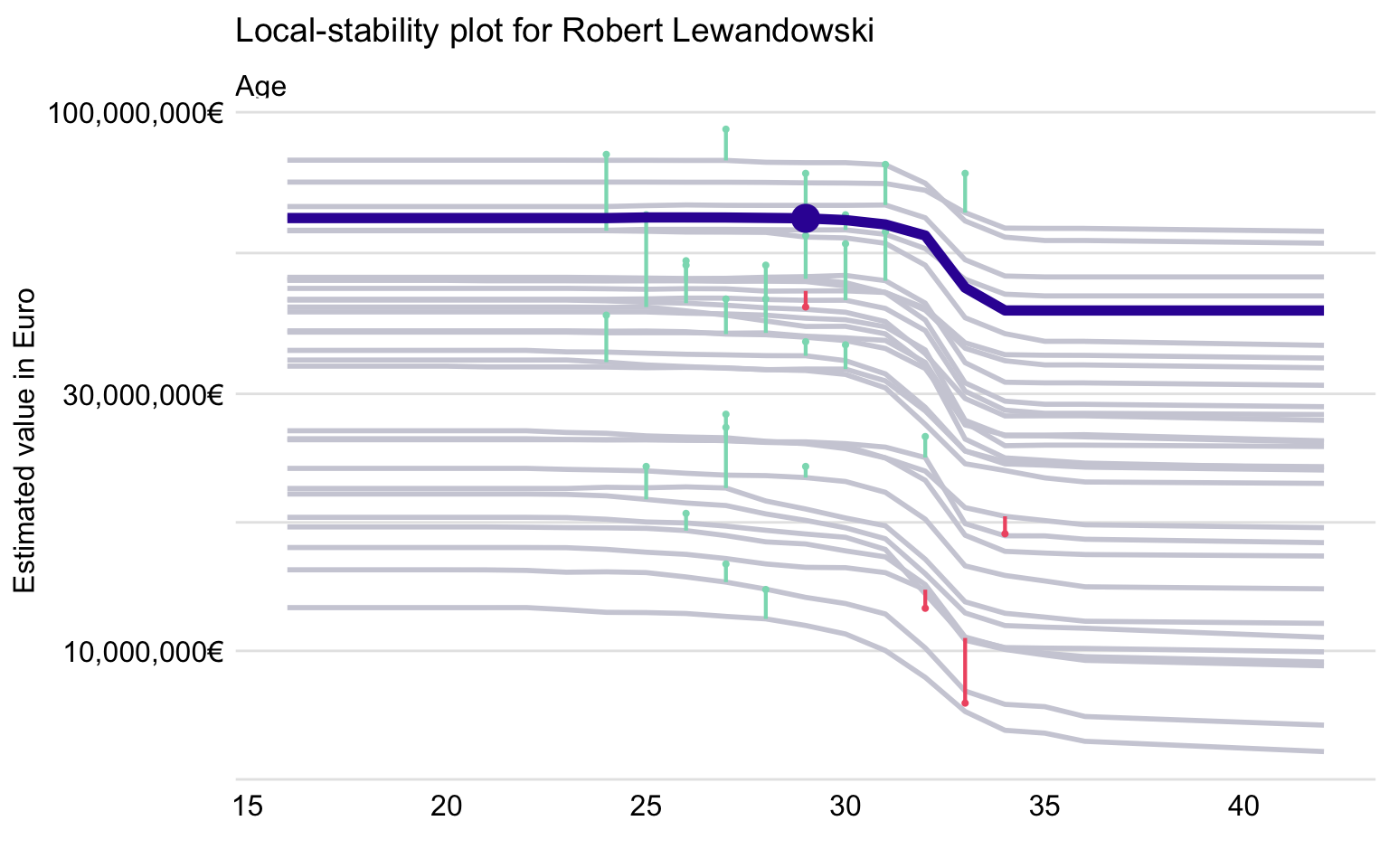
Figure 21.12: Local-stability plot for Age for 30 neighbors of Robert Lewandowski and the random forest model.
The CP profiles in Figure 21.12 are almost parallel but span quite a wide range of the predicted player’s values. Thus, one could conclude that the predictions for the most expensive players are not very stable. Also, the plot includes more positive residuals (indicated in the plot by green vertical intervals) than negative ones (indicated by red vertical intervals). This confirms the conclusion drawn from Figure 21.11 that the values of the most expensive players are underestimated by the model.
21.7.2 Code snippets for R
In this section, we show R-code snippets for instance-level exploration for the gradient boosting model. For other models, a similar syntax was used.
The predict_parts() function from the DALEX package (see Chapters 6-8) is used to calculate variable attributions. Note that we apply the type = "break_down" argument to prepare BD plots. The generic plot() function is used to graphically present the plots.
fifa_bd_gbm <- predict_parts(fifa_gbm_exp,
                   new_observation = fifa["R. Lewandowski",],
                   type = "break_down")
plot(fifa_bd_gbm) +
  scale_y_continuous("Predicted value in Euro",
                  labels = dollar_format(suffix = "€", prefix = "")) +
  ggtitle("Break-down plot for Robert Lewandowski","")
Shapley values are computed by applying the type = "shap" argument.
fifa_shap_gbm <- predict_parts(fifa_gbm_exp,
                     new_observation = fifa["R. Lewandowski",],
                     type = "shap")
plot(fifa_shap_gbm, show_boxplots = FALSE) +
  scale_y_continuous("Estimated value in Euro",
                   labels = dollar_format(suffix = "€", prefix = "")) +
  ggtitle("Shapley values for Robert Lewandowski","")
The predict_profile() function from the DALEX package (see Section 10.6) is used to calculate the CP profiles. The generic plot() function is applied to graphically present the profiles.
selected_variables <- c("Reactions", "BallControl", "Dribbling", "Age")
fifa_cp_gbm <- predict_profile(fifa_gbm_exp,
                   new_observation = fifa["R. Lewandowski",],
                         variables = selected_variables)
plot(fifa_cp_gbm, variables = selected_variables)
Finally, the predict_diagnostics() function (see Section 12.6) allows calculating local-stability plots. The generic plot() function can be used to plot these profiles for selected variables.
21.7.3 Code snippets for Python
In this section, we show Python-code snippets for instance-level exploration for the gradient boosting model. For other models, a similar syntax was used.
First, we need to select instance of interest. In this example we will use Cristiano Ronaldo.
The predict_parts() method from the dalex library (see Sections 6.7 and 8.6) can be used to calculate calculate variable attributions. The plot() method with max_vars argument is applied to graphically present the corresponding BD plot for up to 20 variables.
To calculate Shapley values, the predict_parts() method should be applied with the type='shap' argument (see Section 8.6).
The predict_profile() method from the dalex library (see Section 10.7 allows calculation of the CP profiles. The plot() method with the variables argument plots the profiles for selected variables.
21.7.4 CR7
As a second example, we present explanations for the random forest-model’s prediction for Cristiano Ronaldo (CR7). Table 21.4 presents his characteristics, as included in the analyzed dataset. Note that Cristiano Ronaldo, as Robert Lewandowski, is also a striker. It might be thus of interest to compare the characteristics contributing to the model’s predictions for the two players.
| variable | value | variable | value | variable | value | variable | value |
|---|---|---|---|---|---|---|---|
| Age | 33 | Dribbling | 88 | ShotPower | 95 | Composure | 95 |
| Preferred.Foot | 2 | Curve | 81 | Jumping | 95 | Marking | 28 |
| Reputation | 5 | FKAccuracy | 76 | Stamina | 88 | StandingTackle | 31 |
| Weak.Foot | 4 | LongPassing | 77 | Strength | 79 | SlidingTackle | 23 |
| Skill.Moves | 5 | BallControl | 94 | LongShots | 93 | GKDiving | 7 |
| Crossing | 84 | Acceleration | 89 | Aggression | 63 | GKHandling | 11 |
| Finishing | 94 | SprintSpeed | 91 | Interceptions | 29 | GKKicking | 15 |
| HeadingAccuracy | 89 | Agility | 87 | Positioning | 95 | GKPositioning | 14 |
| ShortPassing | 81 | Reactions | 96 | Vision | 82 | GKReflexes | 11 |
| Volleys | 87 | Balance | 70 | Penalties | 85 | LogValue | 8 |
The BD plot for Cristiano Ronaldo is presented in Figure 21.13. It suggests that the explanatory variables with the largest effect are ShotPower, LongShots, Volleys, and Vision.
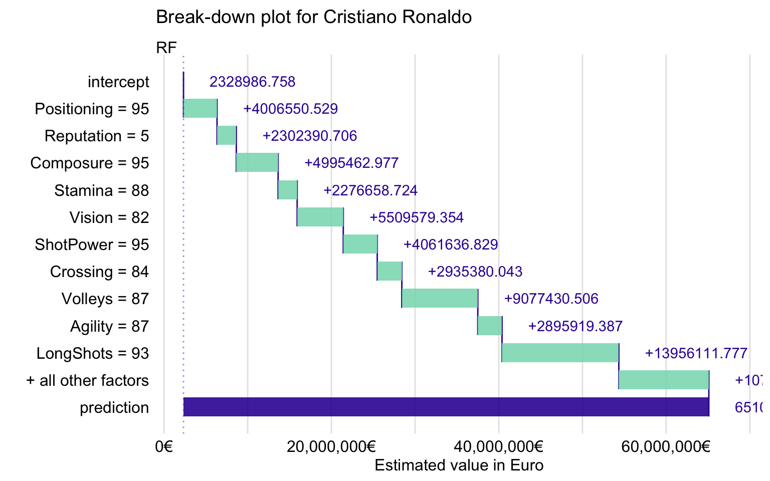
Figure 21.13: Break-down plot for Cristiano Ronaldo for the random forest model.
Figure 21.14 presents Shapley values for Cristiano Ronaldo. It indicates that the four explanatory variables with the largest values are Reactions, Dribbling, BallControl, and ShortPassing. These are the same variables as for Robert Lewandowski, though in a different order. Interestingly, the plot for Cristiano Ronaldo includes variable Age, for which Shapley value is negative. It suggests that CR7’s age has got a negative effect on the model’s prediction.
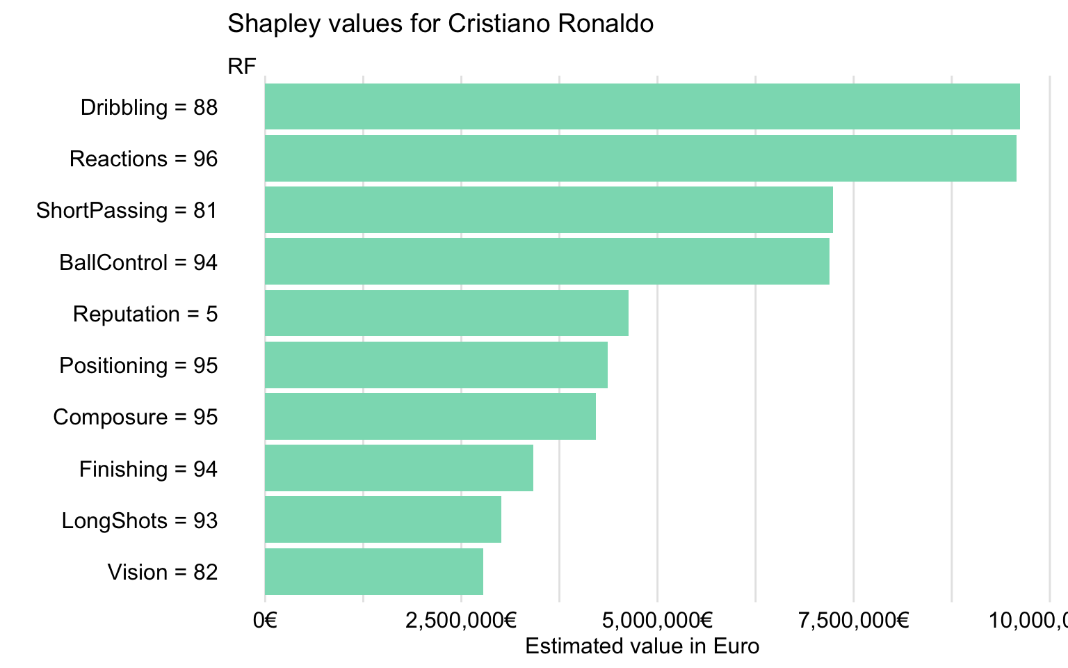
Figure 21.14: Shapley values for Cristiano Ronaldo for the random forest model.
Finally, Figure 21.15 presents CP profiles for Age, Reactions, Dribbling, and BallControl.
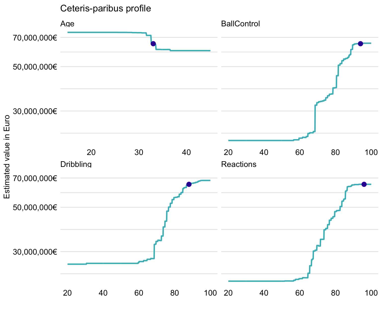
Figure 21.15: Ceteris-paribus profiles for Cristiano Ronaldo for four selected variables and the random forest model.
The profiles are similar to those presented in Figure 21.10 for Robert Lewandowski. An interesting difference is that, for Age, the predicted value for Cristiano Ronaldo is located within the region of age, linked with a sharp drop in player’s value. This is in accordance with the observation, made based on Figure 21.14, that CR7’s age has got a negative effect on the model’s prediction.
21.7.5 Wojciech Szczęsny
One might be interested in the characteristics influencing the random forest model’s predictions for players other than strikers. To address the question, we present explanations for Wojciech Szczęsny, a goalkeeper. Table 21.5 presents his characteristics, as included in the analyzed dataset.
| variable | value | variable | value | variable | value | variable | value |
|---|---|---|---|---|---|---|---|
| Age | 28 | Dribbling | 11 | ShotPower | 15 | Composure | 65 |
| Preferred.Foot | 2 | Curve | 16 | Jumping | 71 | Marking | 20 |
| Reputation | 3 | FKAccuracy | 14 | Stamina | 45 | StandingTackle | 13 |
| Weak.Foot | 3 | LongPassing | 36 | Strength | 65 | SlidingTackle | 12 |
| Skill.Moves | 1 | BallControl | 22 | LongShots | 14 | GKDiving | 85 |
| Crossing | 12 | Acceleration | 51 | Aggression | 40 | GKHandling | 81 |
| Finishing | 12 | SprintSpeed | 47 | Interceptions | 15 | GKKicking | 71 |
| HeadingAccuracy | 16 | Agility | 55 | Positioning | 14 | GKPositioning | 85 |
| ShortPassing | 32 | Reactions | 82 | Vision | 48 | GKReflexes | 87 |
| Volleys | 14 | Balance | 51 | Penalties | 18 | LogValue | 8 |
Figure 21.16 shows the BD plot. We can see that the most important contributions come from the explanatory variables related to goalkeeping skills like GKPositioning, GKHandling, and GKReflexes. Interestingly, field-player skills like BallControl or Dribbling have a negative effect.
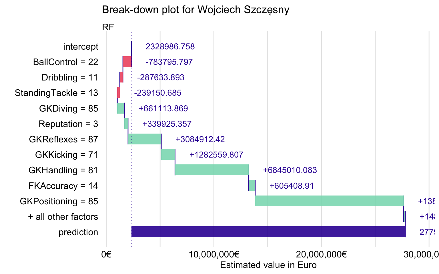
Figure 21.16: Break-down plot for Wojciech Szczęsny for the random forest model.
Figure 21.17 presents Shapley values (over 25 random orderings of explanatory variables). The plot confirms that the most important contributions to the prediction for Wojciech Szczęsny are due to goalkeeping skills like GKDiving, GKPositioning, GKReflexes, and GKHandling. Interestingly, Reactions is also important, as it was the case for Robert Lewandowski (see Figure 21.9) and Cristiano Ronaldo (see Figure 21.14).
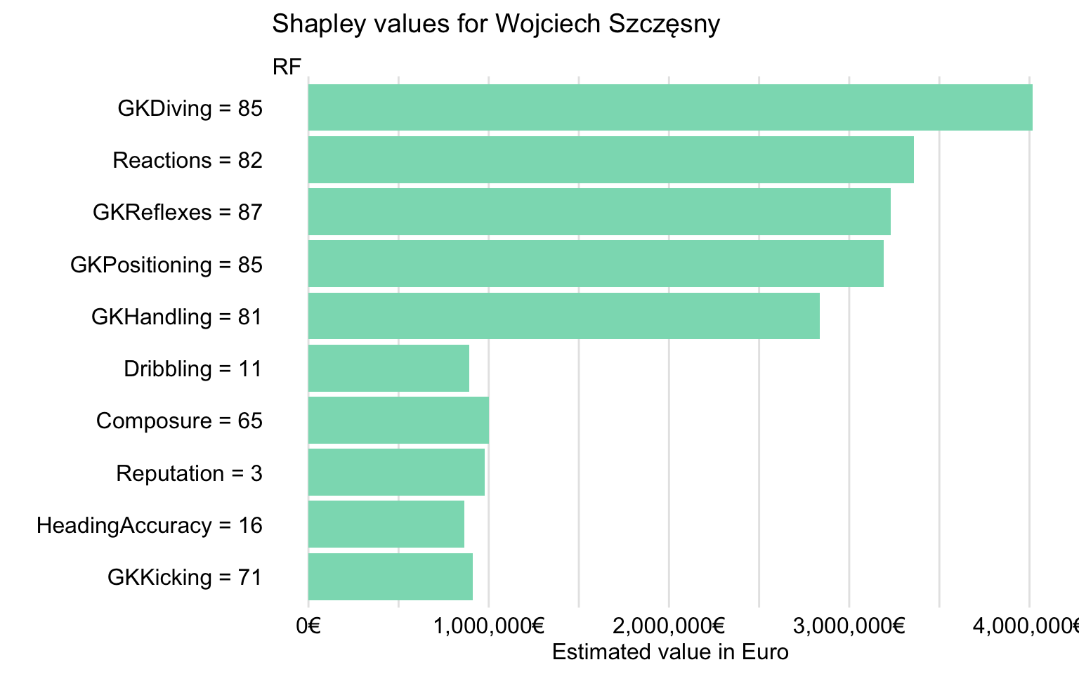
Figure 21.17: Shapley values for Wojciech Szczęsny for the random forest model.
21.7.6 Lionel Messi
This instance might be THE choice for some of the readers. However, we have decided to leave explanation of the models’ predictions in this case as an exercise to the interested readers.
References
Harrell Jr, Frank E. 2018. Rms: Regression Modeling Strategies. https://CRAN.R-project.org/package=rms.
Ridgeway, Greg. 2017. Gbm: Generalized Boosted Regression Models. https://CRAN.R-project.org/package=gbm.
Wright, Marvin N., and Andreas Ziegler. 2017. “ranger: A Fast Implementation of Random Forests for High Dimensional Data in C++ and R.” Journal of Statistical Software 77 (1): 1–17. https://doi.org/10.18637/jss.v077.i01.