8 Shapley Additive Explanations (SHAP) for Average Attributions
In Chapter 6, we introduced break-down (BD) plots, a procedure for calculation of attribution of an explanatory variable for a model’s prediction. We also indicated that, in the presence of interactions, the computed value of the attribution depends on the order of explanatory covariates that are used in calculations. One solution to the problem, presented in Chapter 6, is to find an ordering in which the most important variables are placed at the beginning. Another solution, described in Chapter 7, is to identify interactions and explicitly present their contributions to the predictions.
In this chapter, we introduce yet another approach to address the ordering issue. It is based on the idea of averaging the value of a variable’s attribution over all (or a large number of) possible orderings. The idea is closely linked to “Shapley values” developed originally for cooperative games (Shapley 1953). The approach was first translated to the machine-learning domain by Štrumbelj and Kononenko (2010) and Štrumbelj and Kononenko (2014). It has been widely adopted after the publication of the paper by Lundberg and Lee (2017) and Python’s library for SHapley Additive exPlanations, SHAP (Lundberg 2019). The authors of SHAP introduced an efficient algorithm for tree-based models (Lundberg, Erion, and Lee 2018). They also showed that Shapley values could be presented as a unification of a collection of different commonly used techniques for model explanations (Lundberg and Lee 2017).
8.1 Intuition
Figure 8.1 presents BD plots for 10 random orderings (indicated by the order of the rows in each plot) of explanatory variables for the prediction for Johnny D (see Section 4.2.5) for the random forest model titanic_rf (see Section 4.2.2) for the Titanic dataset. The plots show clear differences in the contributions of various variables for different orderings. The most remarkable differences can be observed for variables fare and class, with contributions changing the sign depending on the ordering.
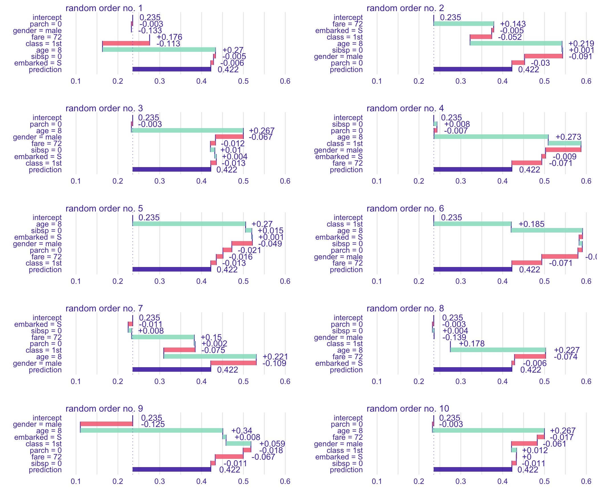
Figure 8.1: Break-down plots for 10 random orderings of explanatory variables for the prediction for Johnny D for the random forest model titanic_rf for the Titanic dataset. Each panel presents a single ordering, indicated by the order of the rows in the plot.
To remove the influence of the ordering of the variables, we can compute the mean value of the attributions. Figure 8.2 presents the averages, calculated over the ten orderings presented in Figure 8.1. Red and green bars present, respectively, the negative and positive averages Violet box plots summarize the distribution of the attributions for each explanatory variable across the different orderings. The plot indicates that the most important variables, from the point of view of the prediction for Johnny D, are age, class, and gender.
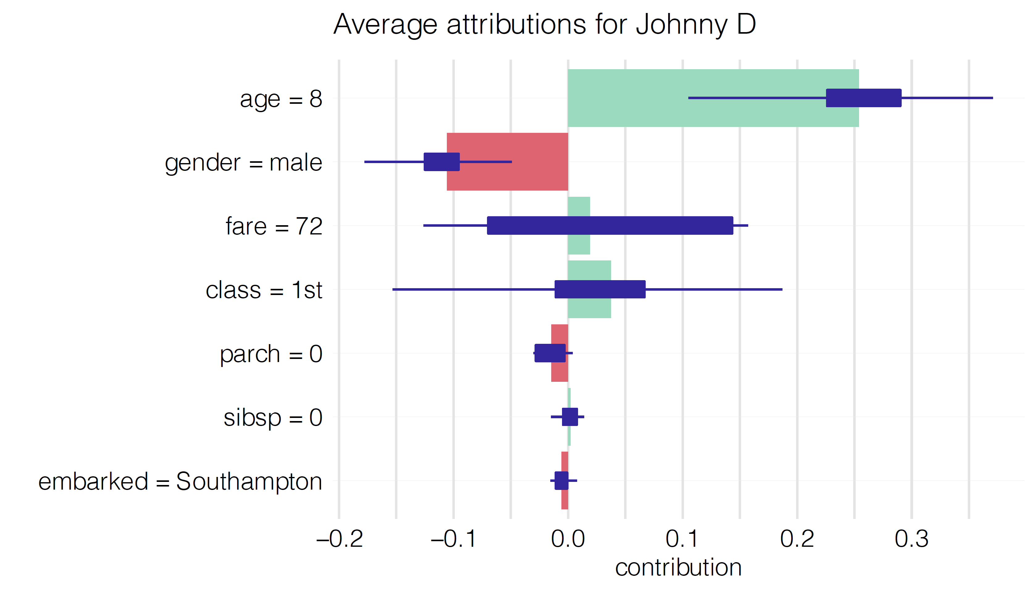
Figure 8.2: Average attributions for 10 random orderings. Red and green bars present the means. Box plots summarize the distribution of contributions for each explanatory variable across the orderings.
8.2 Method
SHapley Additive exPlanations (SHAP) are based on “Shapley values” developed by Shapley (1953) in the cooperative game theory. Note that the terminology may be confusing at first glance. Shapley values are introduced for cooperative games. SHAP is an acronym for a method designed for predictive models. To avoid confusion, we will use the term “Shapley values”.
Shapley values are a solution to the following problem. A coalition of players cooperates and obtains a certain overall gain from the cooperation. Players are not identical, and different players may have different importance. Cooperation is beneficial, because it may bring more benefit than individual actions. The problem to solve is how to distribute the generated surplus among the players. Shapley values offer one possible fair answer to this question (Shapley 1953).
Let’s translate this problem to the context of a model’s predictions. Explanatory variables are the players, while model \(f()\) plays the role of the coalition. The payoff from the coalition is the model’s prediction. The problem to solve is how to distribute the model’s prediction across particular variables?
The idea of using Shapley values for evaluation of local variable-importance was introduced by Štrumbelj and Kononenko (2010). We will define the values using the notation introduced in Section 6.3.2.
Let us consider a permutation \(J\) of the set of indices \(\{1,2,\ldots,p\}\) corresponding to an ordering of \(p\) explanatory variables included in the model \(f()\). Denote by \(\pi(J,j)\) the set of the indices of the variables that are positioned in \(J\) before the \(j\)-th variable. Note that, if the \(j\)-th variable is placed as the first, then \(\pi(J,j) = \emptyset\). Consider the model’s prediction \(f(\underline{x}_*)\) for a particular instance of interest \(\underline{x}_*\). The Shapley value is defined as follows:
\[\begin{equation} \varphi(\underline{x}_*,j) = \frac{1}{p!} \sum_{J} \Delta^{j|\pi(J,j)}(\underline{x}_*), \tag{8.1} \end{equation}\]
where the sum is taken over all \(p!\) possible permutations (orderings of explanatory variables) and the variable-importance measure \(\Delta^{j|J}(\underline{x}_*)\) was defined in equation (6.7) in Section 6.3.2. Essentially, \(\varphi(\underline{x}_*,j)\) is the average of the variable-importance measures across all possible orderings of explanatory variables.
It is worth noting that the value of \(\Delta^{j|\pi(J,j)}(\underline{x}_*)\) is constant for all permutations \(J\) that share the same subset \(\pi(J,j)\). It follows that equation (8.1) can be expressed in an alternative form:
\[\begin{eqnarray} \varphi(\underline{x}_*,j) &=& \frac 1{p!}\sum_{s=0}^{p-1} \sum_{ \substack{ S \subseteq \{1,\ldots,p\}\setminus \{j\} \\ |S|=s }} \left\{s!(p-1-s)! \Delta^{j|S}(\underline{x}_*)\right\}\nonumber\\ &=& \frac 1{p}\sum_{s=0}^{p-1} \sum_{ \substack{ S \subseteq \{1,\ldots,p\}\setminus \{j\} \\ |S|=s }} \left\{{{p-1}\choose{s}}^{-1} \Delta^{j|S}(\underline{x}_*)\right\}, \tag{8.2} \end{eqnarray}\]
where \(|S|\) denotes the cardinal number (size) of set \(S\) and the second sum is taken over all subsets \(S\) of explanatory variables, excluding the \(j\)-th one, of size \(s\).
Note that the number of all subsets of sizes from 0 to \(p-1\) is \(2^{p}-1\), i.e., it is much smaller than number of all permutations \(p!\). Nevertheless, for a large \(p\), it may be feasible to compute Shapley values neither using (8.1) nor (8.2). In that case, an estimate based on a sample of permutations may be considered. A Monte Carlo estimator was introduced by Štrumbelj and Kononenko (2014). An efficient implementation of computations of Shapley values for tree-based models was used in package SHAP (Lundberg and Lee 2017).
From the properties of Shapley values for cooperative games it follows that, in the context of predictive models, they enjoy the following properties:
Symmetry: if two explanatory variables \(j\) and \(k\) are interchangeable, i.e., if, for any set of explanatory variables \(S \subseteq \{1,\dots,p\}\setminus \{j,k\}\) we have got \[ \Delta^{j|S}(\underline{x}_*) = \Delta^{k|S}(\underline{x}_*), \] then their Shapley values are equal: \[ \varphi(\underline{x}_*,j) = \varphi(\underline{x}_*,k). \]
Dummy feature: if an explanatory variable \(j\) does not contribute to any prediction for any set of explanatory variables \(S \subseteq \{1,\dots,p\}\setminus \{j\}\), that is, if \[ \Delta^{j|S}(\underline{x}_*) = 0, \] then its Shapley value is equal to 0: \[ \varphi(\underline{x}_*,j) = 0. \]
Additivity: if model \(f()\) is a sum of two other models \(g()\) and \(h()\), then the Shapley value calculated for model \(f()\) is a sum of Shapley values for models \(g()\) and \(h()\).
Local accuracy (see Section 6.3.2): the sum of Shapley values is equal to the model’s prediction, that is, \[ f(\underline{x}_*) - E_{\underline{X}}\{f(\underline{X})\} = \sum_{j=1}^p \varphi(\underline{x}_*,j), \] where \(\underline{X}\) is the vector of explanatory variables (corresponding to \(\underline{x}_*\)) that are treated as random values.
8.3 Example: Titanic data
Let us consider the random forest model titanic_rf (see Section 4.2.2) and passenger Johnny D (see Section 4.2.5) as the instance of interest in the Titanic data.
Box plots in Figure 8.3 present the distribution of the contributions \(\Delta^{j|\pi(J,j)}(\underline{x}_*)\) for each explanatory variable of the model for 25 random orderings of the explanatory variables. Red and green bars represent, respectively, the negative and positive Shapley values across the orderings. It is clear that the young age of Johnny D results in a positive contribution for all orderings; the resulting Shapley value is equal to 0.2525. On the other hand, the effect of gender is in all cases negative, with the Shapley value equal to -0.0908.
The picture for variables fare and class is more complex, as their contributions can even change the sign, depending on the ordering. Note that Figure 8.3 presents Shapley values separately for each of the two variables. However, it is worth recalling that the iBD plot in Figure 7.1 indicated an important contribution of an interaction between the two variables. Hence, their contributions should not be separated. Thus, the Shapley values for fare and class, presented in Figure 8.3, should be interpreted with caution.
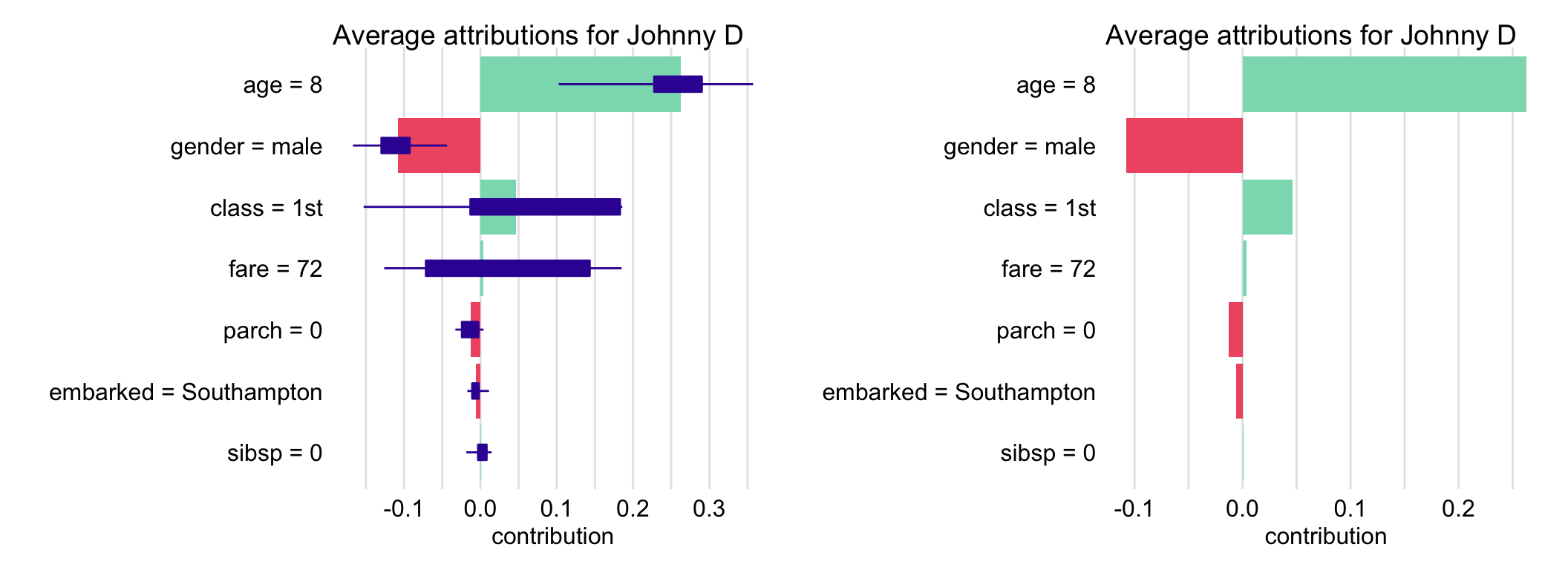
Figure 8.3: Explanatory-variable attributions for the prediction for Johnny D for the random forest model titanic_rf and the Titanic data based on 25 random orderings. Left-hand-side plot: box plots summarize the distribution of the attributions for each explanatory variable across the orderings. Red and green bars present Shapley values. Right-hand-side plot: Shapley values (mean attributions) without box plots.
In most applications, the detailed information about the distribution of variable contributions across the considered orderings of explanatory variables may not be of interest. Thus, one could simplify the plot by presenting only the Shapley values, as illustrated in the right-hand-side panel of Figure 8.3. Table 8.1 presents the Shapley values underlying this plot.
| Variable | Shapley value |
|---|---|
| age = 8 | 0.2525 |
| class = 1st | 0.0246 |
| embarked = Southampton | -0.0032 |
| fare = 72 | 0.0140 |
| gender = male | -0.0943 |
| parch = 0 | -0.0097 |
| sibsp = 0 | 0.0027 |
8.4 Pros and cons
Shapley values provide a uniform approach to decompose a model’s predictions into contributions that can be attributed additively to different explanatory variables. Lundberg and Lee (2017) showed that the method unifies different approaches to additive variable attributions, like DeepLIFT (Shrikumar, Greenside, and Kundaje 2017), Layer-Wise Relevance Propagation (Binder et al. 2016), or Local Interpretable Model-agnostic Explanations (Ribeiro, Singh, and Guestrin 2016). The method has got a strong formal foundation derived from the cooperative games theory. It also enjoys an efficient implementation in Python, with ports or re-implementations in R.
An important drawback of Shapley values is that they provide additive contributions (attributions) of explanatory variables. If the model is not additive, then the Shapley values may be misleading. This issue can be seen as arising from the fact that, in cooperative games, the goal is to distribute the payoff among payers. However, in the predictive modelling context, we want to understand how do the players affect the payoff? Thus, we are not limited to independent payoff-splits for players.
It is worth noting that, for an additive model, the approaches presented in Chapters 6–7 and in the current one lead to the same attributions. The reason is that, for additive models, different orderings lead to the same contributions. Since Shapley values can be seen as the mean across all orderings, it is essentially an average of identical values, i.e., it also assumes the same value.
An important practical limitation of the general model-agnostic method is that, for large models, the calculation of Shapley values is time-consuming. However, sub-sampling can be used to address the issue. For tree-based models, effective implementations are available.
8.5 Code snippets for R
In this section, we use the DALEX package, which is a wrapper for the iBreakDown R package. The package covers all methods presented in this chapter. It is available on CRAN and GitHub. Note that there are also other R packages that offer similar functionalities, like iml (Molnar, Bischl, and Casalicchio 2018), fastshap (Greenwell 2020) or shapper (Maksymiuk, Gosiewska, and Biecek 2019), which is a wrapper for the Python library SHAP (Lundberg 2019).
For illustration purposes, we use the titanic_rf random forest model for the Titanic data developed in Section 4.2.2. Recall that the model is developed to predict the probability of survival for passengers of Titanic. Instance-level explanations are calculated for Henry, a 47-year-old passenger that travelled in the first class (see Section 4.2.5).
We first retrieve the titanic_rf model-object and the data frame for Henry via the archivist hooks, as listed in Section 4.2.7. We also retrieve the version of the titanic data with imputed missing values.
titanic_imputed <- archivist::aread("pbiecek/models/27e5c")
titanic_rf <- archivist:: aread("pbiecek/models/4e0fc")
henry <- archivist::aread("pbiecek/models/a6538")
Then we construct the explainer for the model by using function explain() from the DALEX package (see Section 4.2.6). We also load the randomForest package, as the model was fitted by using function randomForest() from this package (see Section 4.2.2) and it is important to have the corresponding predict() function available. The model’s prediction for Henry is obtained with the help of the function.
library("randomForest")
library("DALEX")
explain_rf <- DALEX::explain(model = titanic_rf,
                        data = titanic_imputed[, -9],
                           y = titanic_imputed$survived == "yes",
                       label = "Random Forest")
predict(explain_rf, henry)
## [1] 0.246To compute Shapley values for Henry, we apply function predict_parts() (as in Section 6.6) to the explainer-object explain_rf and the data frame for the instance of interest, i.e., Henry. By specifying the type="shap" argument we indicate that we want to compute Shapley values. Additionally, the B=25 argument indicates that we want to select 25 random orderings of explanatory variables for which the Shapley values are to be computed. Note that B=25 is also the default value of the argument.
The resulting object shap_henry is a data frame with variable-specific attributions computed for every ordering. Printing out the object provides various summary statistics of the attributions including, of course, the mean.
##                                             min           q1
## Random Forest: age = 47             -0.14872225 -0.081197100
## Random Forest: class = 1st           0.12112732  0.123195061
## Random Forest: embarked = Cherbourg  0.01245129  0.022680335
## Random Forest: fare = 25            -0.03180517 -0.011710693
## Random Forest: gender = male        -0.15670412 -0.145184866
## Random Forest: parch = 0            -0.02795650 -0.007438151
## Random Forest: sibsp = 0            -0.03593203 -0.012978704
##                                           median         mean
## Random Forest: age = 47             -0.040909832 -0.060137381
## Random Forest: class = 1st           0.159974789  0.159090494
## Random Forest: embarked = Cherbourg  0.045746262  0.051056420
## Random Forest: fare = 25            -0.008647485  0.002175261
## Random Forest: gender = male        -0.126003135 -0.126984069
## Random Forest: parch = 0            -0.003043951 -0.005439239
## Random Forest: sibsp = 0            -0.005466244 -0.009070956
##                                                q3          max
## Random Forest: age = 47             -0.0230765745 -0.004967830
## Random Forest: class = 1st           0.1851354780  0.232307204
## Random Forest: embarked = Cherbourg  0.0558871772  0.117857725
## Random Forest: fare = 25             0.0162267784  0.070487540
## Random Forest: gender = male        -0.1115160852 -0.101295877
## Random Forest: parch = 0            -0.0008337109  0.003412778
## Random Forest: sibsp = 0             0.0031207522  0.007650204
By applying the generic function plot() to the shap_henry object, we obtain a graphical illustration of the results.
The resulting plot is shown in Figure 8.4. It includes the Shapley values and box plots summarizing the distributions of the variable-specific contributions for the selected random orderings.
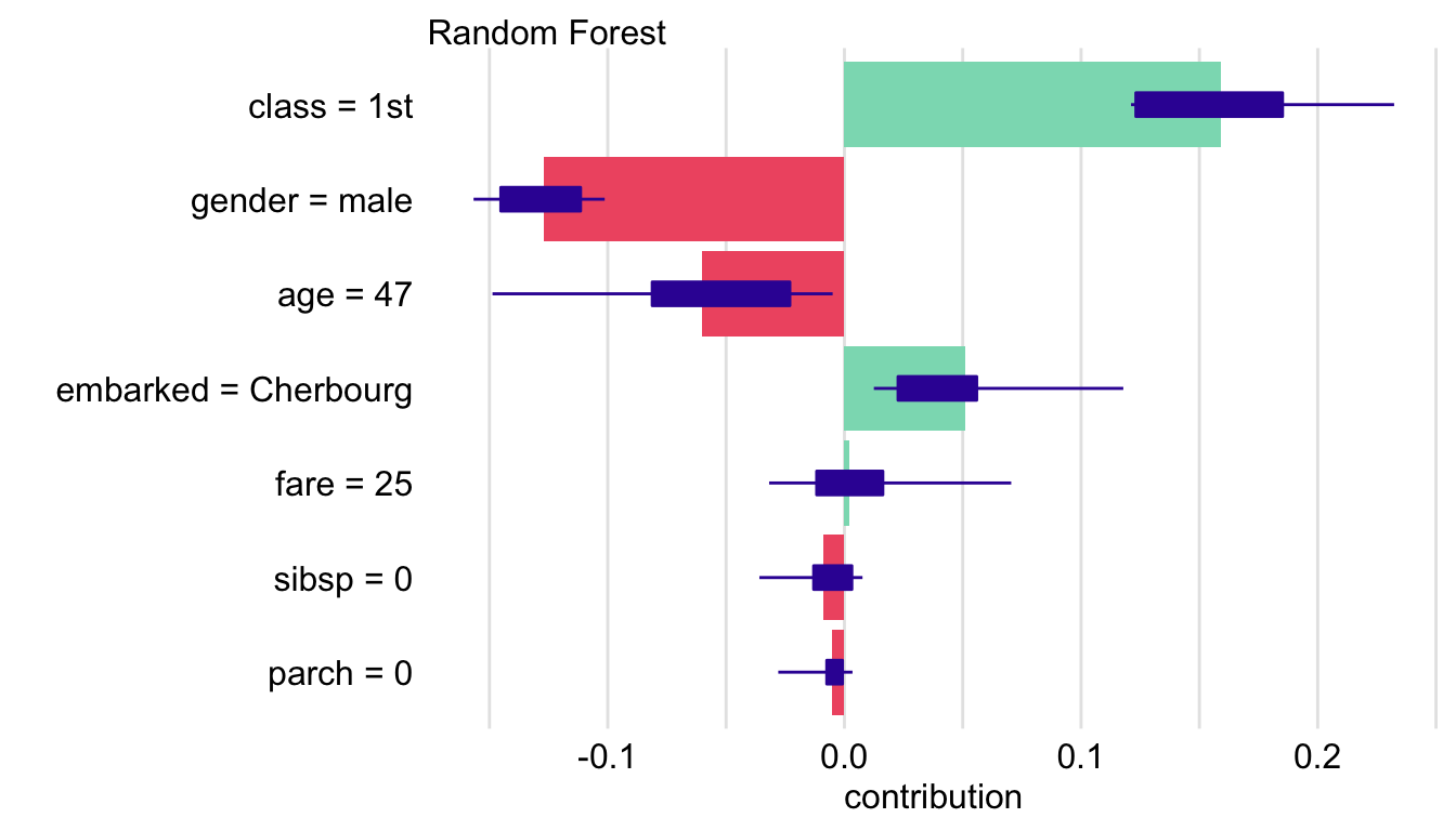
Figure 8.4: A plot of Shapley values with box plots for the titanic_rf model and passenger Henry for the Titanic data, obtained by applying the generic plot() function in R.
To obtain a plot with only Shapley values, i.e., without the box plots, we apply the show_boxplots=FALSE argument in the plot() function call.
The resulting plot, shown in Figure 8.5, can be compared to the plot in the right-hand-side panel of Figure 8.3 for Johnny D. The most remarkable difference is related to the contribution of age. The young age of Johnny D markedly increases the chances of survival, contrary to the negative contribution of the age of 47 for Henry.
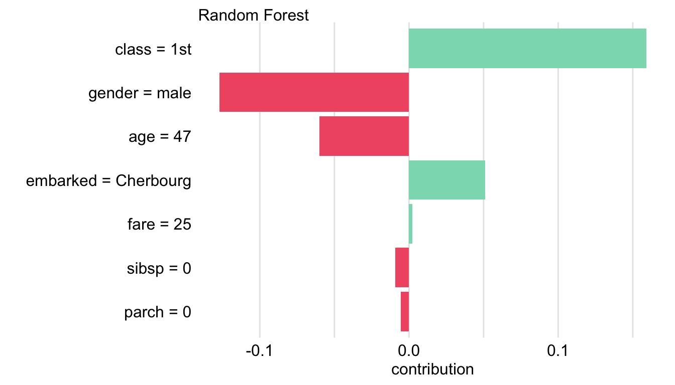
Figure 8.5: A plot of Shapley values without box plots for the titanic_rf model and passenger Henry for the Titanic data, obtained by applying the generic plot() function in R.
8.6 Code snippets for Python
In this section, we use the dalex library for Python. The package covers all methods presented in this chapter. It is available on pip and GitHub. Note that the most popular implementation in Python is available in the shap library (Lundberg and Lee 2017). In this section, however, we show implementations from the dalex library because they are consistent with other methods presented in this book.
For illustration purposes, we use the titanic_rf random forest model for the Titanic data developed in Section 4.3.2. Instance-level explanations are calculated for Henry, a 47-year-old passenger that travelled in the 1st class (see Section 4.3.5).
In the first step, we create an explainer-object that provides a uniform interface for the predictive model. We use the Explainer() constructor for this purpose (see Section 4.3.6).
import pandas as pd
henry = pd.DataFrame({'gender'   : ['male'],
                       'age'     : [47],
                       'class'   : ['1st'],
                       'embarked': ['Cherbourg'],
                       'fare'    : [25],
                       'sibsp'   : [0],
                       'parch'   : [0]},
                      index = ['Henry'])

import dalex as dx
titanic_rf_exp = dx.Explainer(titanic_rf, X, y,
                  label = "Titanic RF Pipeline")
To calculate Shapley values we use the predict_parts() method with the type='shap' argument (see Section 6.7). The first argument indicates the data observation for which the values are to be calculated. Results are stored in the results field.
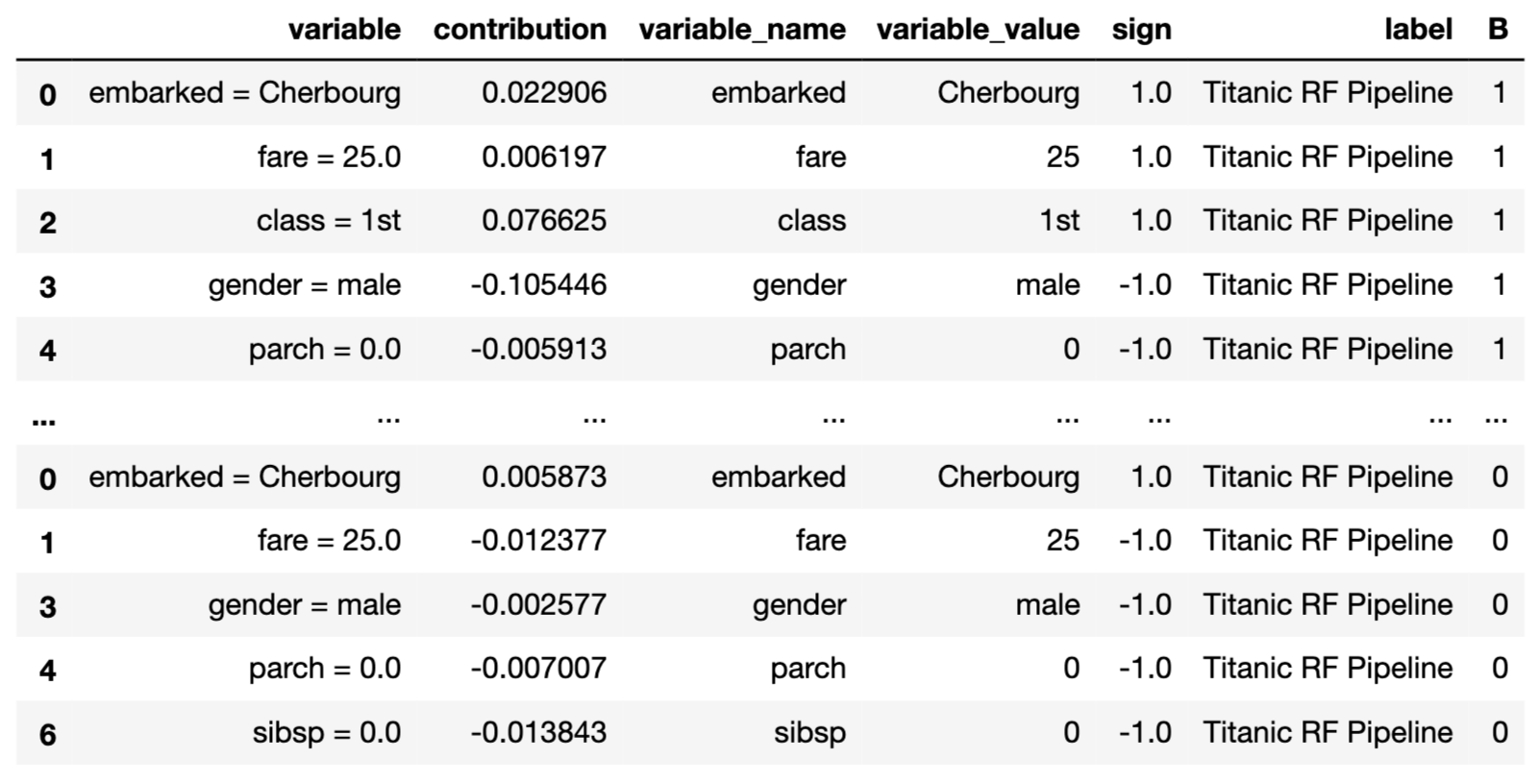
To visualize the obtained values, we simply call the plot() method.
The resulting plot is shown in Figure 8.6.
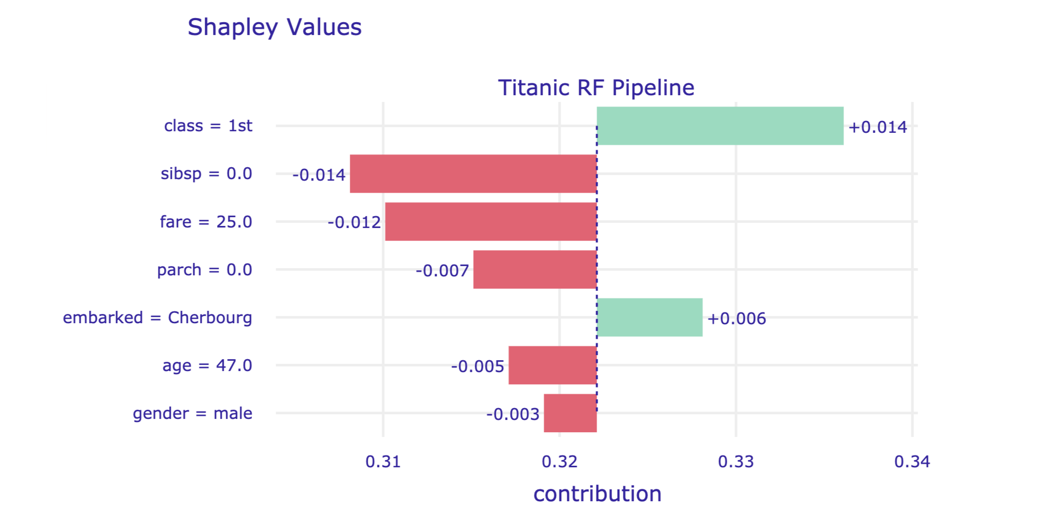
Figure 8.6: A plot of Shapley values for the titanic_rf model and passenger Henry for the Titanic data, obtained by applying the plot() method in Python.
By default, Shapley values are calculated and plotted for all variables in the data. To limit the number of variables included in the graph, we can use the argument max_vars in the plot() method (see Section 6.7).
References
Binder, Alexander, Grégoire Montavon, Sebastian Bach, Klaus-Robert Müller, and Wojciech Samek. 2016. “Layer-Wise Relevance Propagation for Neural Networks with Local Renormalization Layers.” In Artificial Neural Networks and Machine Learning - 25th International Conference on Artificial Neural Networks, Icann 2016, Proceedings, 9887 LNCS:63–71. Lecture Notes in Computer Science. Springer Verlag. https://doi.org/10.1007/978-3-319-44781-0_8.
Greenwell, Brandon. 2020. fastshap: Fast Approximate Shapley Values. https://CRAN.R-project.org/package=fastshap.
Lundberg, Scott. 2019. SHAP (SHapley Additive exPlanations). https://github.com/slundberg/shap.
Lundberg, Scott M., Gabriel G. Erion, and Su-In Lee. 2018. “Consistent Individualized Feature Attribution for Tree Ensembles.” CoRR abs/1802.03888. http://arxiv.org/abs/1802.03888.
Lundberg, Scott M, and Su-In Lee. 2017. “A Unified Approach to Interpreting Model Predictions.” In Advances in Neural Information Processing Systems 30, edited by I. Guyon, U. V. Luxburg, S. Bengio, H. Wallach, R. Fergus, S. Vishwanathan, and R. Garnett, 4765–74. Montreal: Curran Associates. http://papers.nips.cc/paper/7062-a-unified-approach-to-interpreting-model-predictions.pdf.
Maksymiuk, Szymon, Alicja Gosiewska, and Przemyslaw Biecek. 2019. shapper: Wrapper of Python library shap. https://github.com/ModelOriented/shapper.
Molnar, Christoph, Bernd Bischl, and Giuseppe Casalicchio. 2018. “iml: An R package for Interpretable Machine Learning.” Journal of Open Source Software 3 (26): 786. https://doi.org/10.21105/joss.00786.
Ribeiro, Marco Tulio, Sameer Singh, and Carlos Guestrin. 2016. “"Why should I trust you?": Explaining the Predictions of Any Classifier.” In Proceedings of the 22nd ACM SIGKDD International Conference on Knowledge Discovery and Data Mining, Kdd San Francisco, ca, 1135–44. New York, NY: Association for Computing Machinery.
Shapley, Lloyd S. 1953. “A Value for n-Person Games.” In Contributions to the Theory of Games Ii, edited by Harold W. Kuhn and Albert W. Tucker, 307–17. Princeton: Princeton University Press.
Shrikumar, Avanti, Peyton Greenside, and Anshul Kundaje. 2017. “Learning Important Features Through Propagating Activation Differences.” In ICML, edited by Doina Precup and Yee Whye Teh, 70:3145–53. Proceedings of Machine Learning Research. http://dblp.uni-trier.de/db/conf/icml/icml2017.html#ShrikumarGK17.
Štrumbelj, Erik, and Igor Kononenko. 2010. “An Efficient Explanation of Individual Classifications Using Game Theory.” Journal of Machine Learning Research 11 (March): 1–18. http://dl.acm.org/citation.cfm?id=1756006.1756007.
Štrumbelj, Erik, and Igor Kononenko. 2014. “Explaining prediction models and individual predictions with feature contributions.” Knowledge and Information Systems 41 (3): 647–65. https://doi.org/10.1007/s10115-013-0679-x.