18 Local-dependence and Accumulated-local Profiles

18.1 Introduction

Partial-dependence (PD) profiles, introduced in the previous chapter, are easy to explain and interpret, especially given their estimation as the mean of ceteris-paribus (CP) profiles. However, as it was mentioned in Section 17.5, the profiles may be misleading if, for instance, explanatory variables are correlated. In many applications, this is the case. For example, in the apartment-prices dataset (see Section 4.4), one can expect that variables surface and number of rooms may be positively correlated, because apartments with a larger number of rooms usually also have a larger surface. Thus, in ceteris-paribus profiles, it is not realistic to consider, for instance, an apartment with five rooms and a surface of 20 square meters. Similarly, in the Titanic dataset, a positive association can be expected for the values of variables fare and class, as tickets in the higher classes are more expensive than in the lower classes.

In this chapter, we present accumulated-local profiles that address this issue. As they are related to local-dependence profiles, we introduce the latter first. Both approaches were proposed by Apley (2018).

18.2 Intuition

Let us consider the following simple linear model with two explanatory variables:

\[\begin{equation} Y = X^1 + X^2 + \varepsilon = f(X^1, X^2) + \varepsilon, \tag{18.1} \end{equation}\]

where \(\varepsilon \sim N(0,0.1^2)\).

For this model, the effect of \(X^1\) for any value of \(X^2\) is linear, i.e., it can be described by a straight line with the intercept equal to 0 and the slope equal to 1.

Assume that observations of explanatory variables \(X^1\) and \(X^2\) are uniformly distributed over the unit square, as illustrated in the left-hand-side panel of Figure 18.1 for a set of 1000 observations. The right-hand-side panel of Figure 18.1 presents the scatter plot of the observed values of \(Y\) in function of \(X^1\). The plot for \(X^2\) is, essentially, the same and we do not show it.

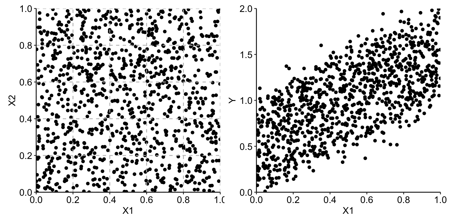
Figure 18.1: Observations of two explanatory variables uniformly distributed over the unit square (left-hand-side panel) and the scatter plot of the observed values of the dependent variable \(Y\) in function of \(X^1\) (right-hand-side panel).

In view of the plot shown in the right-hand-side panel of Figure 18.1, we could consider using a simple linear model with \(X^1\) and \(X^2\) as explanatory variables. Assume, however, that we would like to analyze the data without postulating any particular parametric form of the effect of the variables. A naïve way would be to split the observed range of each of the two variables into, for instance, five intervals (as illustrated in the left-hand-side panel of Figure 18.1), and estimate the means of observed values of \(Y\) for the resulting 25 groups of observations. Table 18.1 presents the sample means (with rows and columns defined by the ranges of possible values of, respectively, \(X^1\) and \(X^2\)).

Table 18.1: Sample means of \(Y\) for 25 groups of observations resulting from splitting the ranges of explanatory variables \(X^1\) and \(X^2\) into five intervals (see the left-hand-side panel of Figure 18.1).

	(0,0.2]	(0.2,0.4]	(0.4,0.6]	(0.6,0.8]	(0.8,1]
(0,0.2]	0.19	0.42	0.63	0.80	0.99
(0.2,0.4]	0.39	0.59	0.81	1.01	1.19
(0.4,0.6]	0.59	0.81	0.98	1.20	1.44
(0.6,0.8]	0.76	1.00	1.20	1.40	1.58
(0.8,1]	1.01	1.22	1.38	1.58	1.77

Table 18.2 presents the number of observations for each of the sample means from Table 18.1.

Table 18.2: Number of observations for the sample means from Table 18.1.

	(0,0.2]	(0.2,0.4]	(0.4,0.6]	(0.6,0.8]	(0.8,1]	total
(0,0.2]	51	39	31	43	43	207
(0.2,0.4]	39	40	35	53	42	209
(0.4,0.6]	28	42	35	49	40	194
(0.6,0.8]	37	30	36	55	45	203
(0.8,1]	43	46	36	28	34	187
total	198	197	173	228	204	1000

By using this simple approach, we can compute the PD profile for \(X^1\). Consider \(X^1=z\). To apply the estimator defined in (17.2), we need the predicted values \(\hat{f}(z,x^2_i)\) for any observed value of \(x^2_i \in [0,1]\). As our observations are uncorrelated and fill-in the unit-square, we can use the suitable mean values for that purpose. In particular, for \(z \in [0,0.2]\), we get

\[\begin{align} \hat g_{PD}^{1}(z) &= \frac{1}{1000}\sum_{i}\hat{f}(z,x^2_i) = \nonumber \\ &= (198\times 0.19 + 197\times 0.42 + 173\times 0.63 + \nonumber\\ & \ \ \ \ \ 228\times 0.80 + 204\times 1.00)/1000 = 0.6. \nonumber \tag{18.2} \end{align}\]

By following the same principle, for \(z \in (0.2,0.4]\), \((0.4,0.6]\), \((0.6,0.8]\), and \((0.8,1]\) we get the values of 0.8, 1, 1.2, and 1.4, respectively. Thus, overall, we obtain a piecewise-constant profile with values that capture the (correct) linear effect of \(X^1\) in model (18.1). In fact, by using, for instance, midpoints of the intervals for \(z\), i.e., 0.1, 0.3, 0.5, 0.7, and 0.9, we could describe the profile by the linear function \(0.5+z\).

Assume now that we are given the data only from the regions on the diagonal of the unit square, as illustrated in the left-hand-side panel of Figure 18.2. In that case, the observed values of \(X^1\) and \(X^2\) are strongly correlated, with the estimated value of Pearson’s correlation coefficient equal to 0.96. The right-hand-side panel of Figure 18.2 presents the scatter plot of the observed values of \(Y\) in the function of \(X^1\).

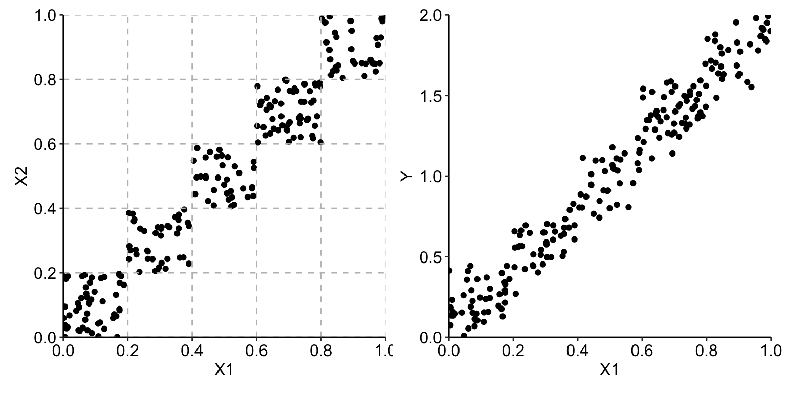
Figure 18.2: Correlated observations of two explanatory variables (left-hand-side panel) and the scatter plot of the observed values of the dependent variable \(Y\) in the function of \(X^1\) (right-hand-side panel).

Now, the “naïve” modelling approach would amount to using only five sample means, as in the table below.

Table 18.3: Sample means of \(Y\) for five groups of observations (see the left-hand-side panel of Figure 18.2).

	(0,0.2]	(0.2,0.4]	(0.4,0.6]	(0.6,0.8]	(0.8,1]
(0,0.2]	0.19	NA	NA	NA	NA
(0.2,0.4]	NA	0.59	NA	NA	NA
(0.4,0.6]	NA	NA	0.98	NA	NA
(0.6,0.8]	NA	NA	NA	1.4	NA
(0.8,1]	NA	NA	NA	NA	1.77

When computing the PD profile for \(X^1\), we now encounter the issue related to the fact that, for instance, for \(z \in [0,0.2]\), we have not got any observations and, hence, any sample mean for \(x^2_i>0.2\). To overcome this issue, we could extrapolate the predictions (i.e., mean values) obtained for other intervals of \(z\). That is, we could assume that, for \(x^2_i \in (0.2,0.4]\), the prediction is equal to 0.59, for \(x^2_i \in (0.4,0.6]\) it is equal to 0.98, and so on. This leads to the following value of the PD profile for \(z \in [0,0.2]\):

\[\begin{align} \hat g_{PD}^{1}(z) &= \frac{1}{51 + 40 + 35 + 55 + 34}\sum_{i}\hat{f}(z,x^2_i) = \nonumber \\ &= \frac{1}{215}(51\times0.19 + 40\times0.59 + 35\times0.98 + \nonumber \\ & \ \ \ \ \ 55\times1.40 + 34\times1.77)=0.95. \end{align}\]

This is a larger value than 0.6 computed in (18.2) for the uncorrelated data. The reason is the extrapolation: for instance, for \(z \in [0,0.2]\) and \(x^2_i \in (0.6,0.8]\), we use 1.40 as the predicted value of \(Y\). However, Table 18.1 indicates that the sample mean for those observations is equal to 0.80.

In fact, by using the same extrapolation principle, we get \(\hat g_{PD}^{1}(z) = 0.95\) also for \(z \in (0.2,0.4]\), \((0.4,0.6]\), \((0.6,0.8]\), and \((0.8,1]\). Thus, the obtained profile indicates no effect of \(X^1\), which is clearly a wrong conclusion.

While the modelling approach presented in the example above may seem to be simplistic, it does illustrate the issue that would also appear for other flexible modelling methods like, for instance, regression trees. In particular, the left-hand-side panel of Figure 18.3 presents a regression tree fitted to the data shown in Figure 18.2 by using function tree() from the R package tree. The right-hand-side panel of Figure 18.3 presents the corresponding split of the observations. According to the model, the predicted value of \(Y\) for the observations in the region \(x^1 \in [0,0.2]\) and \(x^2 \in [0.8,1]\) would be equal to 1.74. This extrapolation implies a substantial overestimation, as the true expected value of \(Y\) in the region is equal to 1. Note that the latter is well estimated by the sample mean equal to 0.99 (see Table 18.1) in the case of the uncorrelated data shown in Figure 18.1.

The PD profile for \(X^1\) for the regression tree would be equal to 0.2, 0.8, and 1.5 for \(z \in [0,0.2]\), \((0.2,0.6]\), and \((0.6,1]\), respectively. It does show an effect of \(X^1\), but if we used midpoints of the intervals for \(z\), i.e., 0.1, 0.4, and 0.8, we could (approximately) describe the profile by the linear function \(2z\), i.e., with a slope larger than (the true value of) 1.

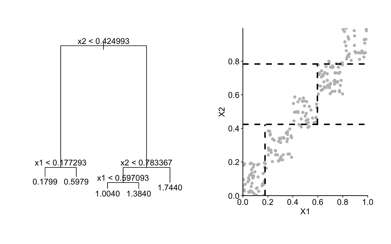
Figure 18.3: Results of fitting of a regression tree to the data shown in Figure 18.2 (left-hand-side panel) and the corresponding split of the observations of the two explanatory variables (right-hand-side panel).

The issue stems from the fact that, in the definition (17.1) of the PD profile, the expected value of model predictions is computed by using the marginal distribution of \(X^2\), which disregards the value of \(X^1\). Clearly, this is an issue when the explanatory variables are correlated. This observation suggests a modification: instead of the marginal distribution, one might use the conditional distribution of \(X^2\) given \(X^1\), because it reflects the association between the two variables. The modification leads to the definition of an LD profile.

It turns out, however, that the modification does not fully address the issue of correlated explanatory variables. As argued by Apley and Zhu (2020), if an explanatory variable is correlated with some other variables, the LD profile for the variable will still capture the effect of the other variables. This is because the profile is obtained by marginalizing over (in fact, ignoring) the remaining variables in the model, which results in an effect similar to the “omitted variable” bias in linear regression. Thus, in this respect, LD profiles share the same limitation as PD profiles. To address the limitation, Apley and Zhu (2020) proposed the concept of local-dependence effects and accumulated-local (AL) profiles.

18.3 Method

18.3.1 Local-dependence profile

Local-dependence (LD) profile for model \(f()\) and variable \(X^j\) is defined as follows:

\[\begin{equation} g_{LD}^{f, j}(z) = E_{\underline{X}^{-j}|X^j=z}\left\{f\left(\underline{X}^{j|=z}\right)\right\}. \tag{18.3} \end{equation}\]

Thus, it is the expected value of the model predictions over the conditional distribution of \(\underline{X}^{-j}\) given \(X^j=z\), i.e., over the joint distribution of all explanatory variables other than \(X^j\) conditional on the value of the latter variable set to \(z\). Or, in other words, it is the expected value of the CP profiles for \(X^j\), defined in (10.1), over the conditional distribution of \(\underline{X}^{-j} | X^j = z\).

As proposed by Apley and Zhu (2020), LD profile can be estimated as follows:

\[\begin{equation} \hat g_{LD}^{j}(z) = \frac{1}{|N_j|} \sum_{k\in N_j} f\left(\underline{x}_k^{j| = z}\right), \tag{18.4} \end{equation}\]

where \(N_j\) is the set of observations with the value of \(X^j\) “close” to \(z\) that is used to estimate the conditional distribution of \(\underline{X}^{-j}|X^j=z\).

Note that, in general, the estimator given in (18.4) is neither smooth nor continuous at boundaries between subsets \(N_j\). A smooth estimator for \(g_{LD}^{f,j}(z)\) can be defined as follows:

\[\begin{equation} \tilde g_{LD}^{j}(z) = \frac{1}{\sum_k w_{k}(z)} \sum_{i = 1}^n w_i(z) f\left(\underline{x}_i^{j| = z}\right), \tag{18.5} \end{equation}\]

where weights \(w_i(z)\) capture the distance between \(z\) and \(x_i^j\). In particular, for a categorical variable, we may just use the indicator function \(w_i(z) = 1_{z = x^j_i}\), while for a continuous variable we may use the Gaussian kernel:

\[\begin{equation} w_i(z) = \phi(z - x_i^j, 0, s), \tag{18.6} \end{equation}\]

where \(\phi(y,0,s)\) is the density of a normal distribution with mean 0 and standard deviation \(s\). Note that \(s\) plays the role of a smoothing factor.

As already mentioned in Section 18.2, if an explanatory variable is correlated with some other variables, the LD profile for the variable will capture the effect of all of the variables. For instance, consider model (18.1). Assume that \(X^1\) has a uniform distribution on \([0,1]\) and that \(X^1=X^2\), i.e., explanatory variables are perfectly correlated. In that case, the LD profile for \(X^1\) is given by

\[ g_{LD}^{1}(z) = E_{X^2|X^1=z}(z+X^2) = z + E_{X^2|X^1=z}(X^2) = 2z. \] Hence, it suggests an effect of \(X^1\) twice larger than the correct one.

To address the limitation, AL profiles can be used. We present them in the next section.

18.3.2 Accumulated-local profile

Consider model \(f()\) and define

\[ q^j(\underline{u})=\left\{ \frac{\partial f(\underline{x})}{\partial x^j} \right\}_{\underline{x}=\underline{u}}. \] Accumulated-local (AL) profile for model \(f()\) and variable \(X^j\) is defined as follows:

\[\begin{equation} g_{AL}^{j}(z) = \int_{z_0}^z \left[E_{\underline{X}^{-j}|X^j=v}\left\{ q^j(\underline{X}^{j|=v}) \right\}\right] dv + c, \tag{18.7} \end{equation}\]

where \(z_0\) is a value close to the lower bound of the effective support of the distribution of \(X^j\) and \(c\) is a constant, usually selected so that \(E_{X^j}\left\{g_{AL}^{j}(X^j)\right\} = 0\).

To interpret (18.7), note that \(q^j(\underline{x}^{j|=v})\) describes the local effect (change) of the model due to \(X^j\). Or, to put it in other words, \(q^j(\underline{x}^{j|=v})\) describes how much the CP profile for \(X^j\) changes at \((x^1,\ldots,x^{j-1},v,x^{j+1},\ldots,x^p)\). This effect (change) is averaged over the “relevant” (according to the conditional distribution of \(\underline{X}^{-j}|X^j\)) values of \(\underline{x}^{-j}\) and, subsequently, accumulated (integrated) over values of \(v\) up to \(z\). As argued by Apley and Zhu (2020), the averaging of the local effects allows avoiding the issue, present in the PD and LD profiles, of capturing the effect of other variables in the profile for a particular variable in additive models (without interactions). To see this, one can consider the approximation

\[ f(\underline{x}^{j|=v+dv})-f(\underline{x}^{j|=v}) \approx q^j(\underline{x}^{j|=v})dv, \]

and note that the difference \(f(\underline{x}^{j|=v+dv})-f(\underline{v}^{j|=v})\), for a model without interaction, effectively removes the effect of all variables other than \(X^j\).

For example, consider model (18.1). In that case, \(f(x^1,x^2)=x^1+x^2\) and \(q^1(\underline{u}) = 1\). Thus,

\[ f(u+du,x_2)-f(u,x_2) = (u + du + x^2) - (u + x^2) = du = q^1(u)du. \]

Consequently, irrespective of the joint distribution of \(X^1\) and \(X^2\) and upon setting \(c=z_0\), we get \[ g_{AL}^{1}(z) = \int_{z_0}^z \left\{E_{{X}^{2}|X^1=v}(1)\right\} dv + z_0 = z. \]

To estimate an AL profile, one replaces the integral in (18.7) by a summation and the derivative with a finite difference (Apley and Zhu 2020). In particular, consider a partition of the range of observed values \(x_{i}^j\) of variable \(X^j\) into \(K\) intervals \(N_j(k)=\left(z_{k-1}^j,z_k^j\right]\) (\(k=1,\ldots,K\)). Note that \(z_0^j\) can be chosen just below \(\min(x_1^j,\ldots,x_N^j)\) and \(z_K^j=\max(x_1^j,\ldots,x_N^j)\). Let \(n_j(k)\) denote the number of observations \(x_i^j\) falling into \(N_j(k)\), with \(\sum_{k=1}^K n_j(k)=n\). An estimator of the AL profile for variable \(X^j\) can then be constructed as follows:

\[\begin{equation} \widehat{g}_{AL}^{j}(z) = \sum_{k=1}^{k_j(z)} \frac{1}{n_j(k)} \sum_{i: x_i^j \in N_j(k)} \left\{ f\left(\underline{x}_i^{j| = z_k^j}\right) - f\left(\underline{x}_i^{j| = z_{k-1}^j}\right) \right\} - \hat{c}, \tag{18.8} \end{equation}\]

where \(k_j(z)\) is the index of interval \(N_j(k)\) in which \(z\) falls, i.e., \(z \in N_j\{k_j(z)\}\), and \(\hat{c}\) is selected so that \(\sum_{i=1}^n \widehat{g}_{AL}^{f,j}(x_i^j)=0\).

To interpret (18.8), note that difference \(f\left(\underline{x}_i^{j| = z_k^j}\right) - f\left(\underline{x}_i^{j| = z_{k-1}^j}\right)\) corresponds to the difference of the CP profile for the \(i\)-th observation at the limits of interval \(N_j(k)\). These differences are then averaged across all observations for which the observed value of \(X^j\) falls into the interval and are then accumulated.

Note that, in general, \(\widehat{g}_{AL}^{f,j}(z)\) is not smooth at the boundaries of intervals \(N_j(k)\). A smooth estimate can obtained as follows:

\[\begin{equation} \widetilde{g}_{AL}^{j}(z) = \sum_{k=1}^K \left[ \frac{1}{\sum_{l} w_l(z_k)} \sum_{i=1}^N w_{i}(z_k) \left\{f\left(\underline{x}_i^{j| = z_k}\right) - f\left(\underline{x}_i^{j| = z_k - \Delta}\right)\right\}\right] - \hat{c}, \tag{18.9} \end{equation}\]

where points \(z_k\) (\(k=0, \ldots, K\)) form a uniform grid covering the interval \((z_0,z)\) with step \(\Delta = (z-z_0)/K\), and weight \(w_i(z_k)\) captures the distance between point \(z_k\) and observation \(x_i^j\). In particular, we may use similar weights as in case of (18.5).

18.3.3 Dependence profiles for a model with interaction and correlated explanatory variables: an example

In this section, we illustrate in more detail the behavior of PD, LD, and AL profiles for a model with an interaction between correlated explanatory variables. In particular, let us consider the following simple model for two explanatory variables:

\[\begin{equation} f(X^1, X^2) = (X^1 + 1)\cdot X^2. \tag{18.10} \end{equation}\]

Moreover, assume that explanatory variables \(X^1\) and \(X^2\) are uniformly distributed over the interval \([-1,1]\) and perfectly correlated, i.e., \(X^2 = X^1\). Suppose that we have got a dataset with eight observations as in Table 18.4. Note that, for both \(X^1\) and \(X^2\), the sum of all observed values is equal to 0.

Table 18.4: A sample of eight observations.

i	1	2	3	4	5	6	7	8
\(X^1\)	-1	-0.71	-0.43	-0.14	0.14	0.43	0.71	1
\(X^2\)	-1	-0.71	-0.43	-0.14	0.14	0.43	0.71	1
\(y\)	0	-0.2059	-0.2451	-0.1204	0.1596	0.6149	1.2141	2

Note that PD, LD, AL profiles describe the effect of a variable in isolation from the values of other variables. In model (18.10), the effect of variable \(X^1\) depends on the value of variable \(X^2\). For models with interactions, it is subjective to define what would be the “true” main effect of variable \(X^1\). Complex predictive models often have interactions. By examining the case of model (18.10), we will provide some intuition on how PD, LD and AL profiles may behave in such cases.

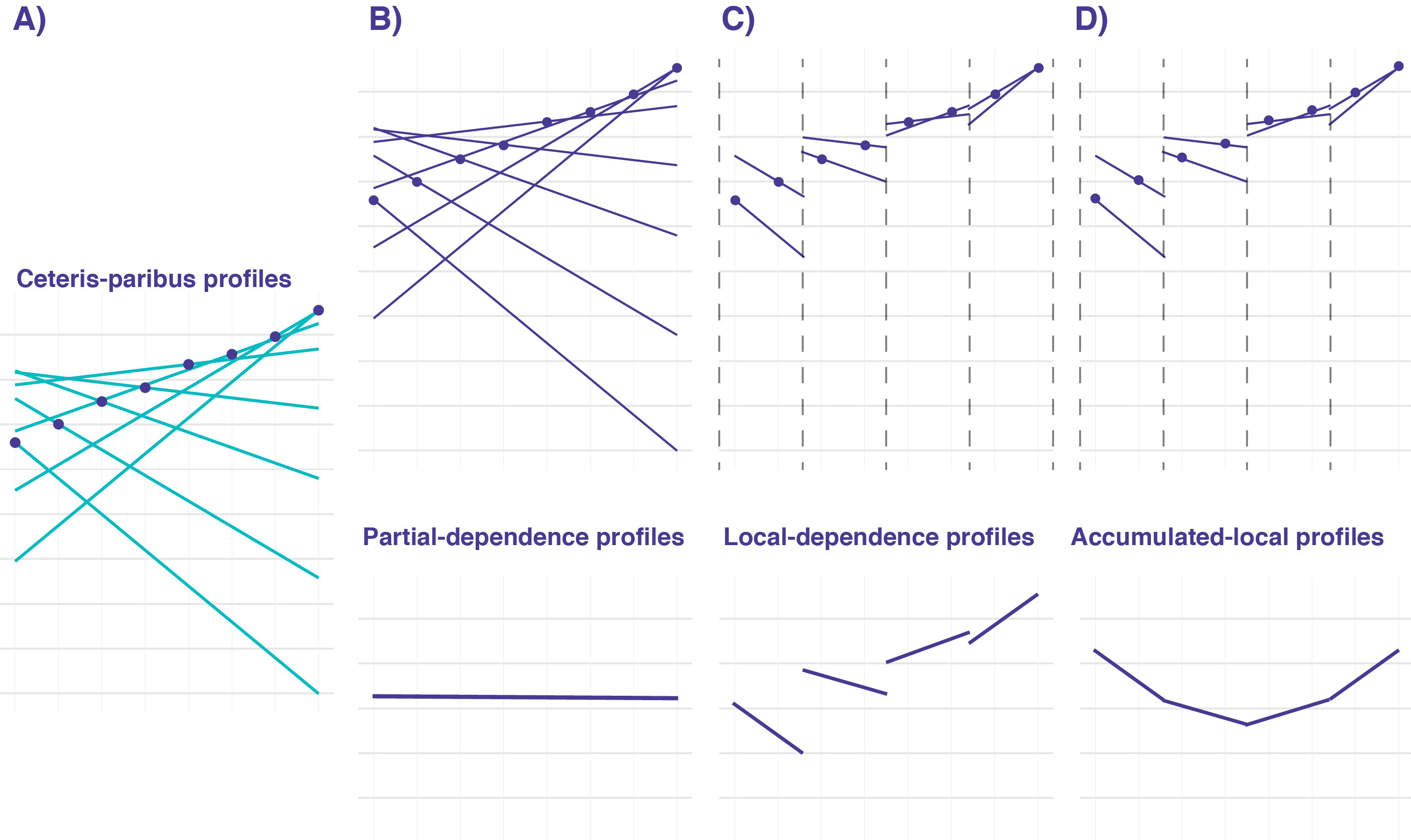
Figure 18.4: Partial-dependence (PD), local-dependence (LD), and accumulated-local (AL) profiles for model (18.10). Panel A: ceteris-paribus (CP) profiles for eight observations from Table 18.4. Panel B: entire CP profiles (top) contribute to calculation of the corresponding PD profile (bottom). Panel C: only parts of the CP profiles (top), close to observations of interest, contribute to the calculation of the corresponding LD profile (bottom). Panel D: only parts of the CP profiles (top) contribute to the calculation of the corresponding AL profile (bottom).

Let us explicitly express the CP profile for \(X^1\) for model (18.10):

\[\begin{equation} h^{1}_{CP}(z) = f(z,X^2) = (z+1)\cdot X^2. \tag{18.11} \end{equation}\]

By allowing \(z\) to take any value in the interval \([-1,1]\), we get the CP profiles as straight lines with the slope equal to the value of variable \(X^2\). Hence, for instance, the CP profile for observation \((-1,-1)\) is a straight line with the slope equal to \(-1\). The CP profiles for the eight observations, from Table 18.4 are presented in panel A of Figure 18.4.

Recall that the PD profile for \(X^j\), defined in equation (17.1), is the expected value, over the joint distribution of all explanatory variables other than \(X^j\), of the model predictions when \(X^j\) is set to \(z\). This leads to the estimation of the profile by taking the average of CP profiles for \(X^j\), as given in (17.2).

In our case, this implies that the PD profile for \(X^1\) is the expected value of the model predictions over the distribution of \(X^2\), i.e., over the uniform distribution on the interval \([-1,1]\). Thus, the PD profile is estimated by taking the average of the CP profiles, given by (18.11), at each value of \(z\) in \([-1,1]\):

\[\begin{equation} \hat g_{PD}^{1}(z) = \frac{1}{8} \sum_{i=1}^{8} (z+1)\cdot X^2_{i} = \frac{z+1}{8} \sum_{i=1}^{8} X^2_{i} = 0. \tag{18.12} \end{equation}\]

As a result, the PD profile for \(X^1\) is estimated as a horizontal line at 0, as seen in the bottom part of Panel B of Figure 18.4.

Since the \(X^1\) and \(X^2\) variables are correlated, it can be argued that we should not include entire CP profiles in the calculation of the PD profile, but only parts of them. In fact, for perfectly correlated explanatory variables, the CP profile for the \(i\)-th observation should actually be undefined for any values of \(z\) different from \(x^2_i\).

The estimated horizontal PD profile results from using the marginal distribution of \(X^2\), which disregards the value of \(X^1\), in the definition of the profile. This observation suggests a modification: instead of the marginal distribution, one might consider the conditional distribution of \(X^2\) given \(X^1\). The modification leads to the definition of LD profile.

For the data from Table 18.4, the conditional distribution of \(X^2\), given \(X^1=z\), is just a probability mass of 1 at \(z\). Consequently, for model (18.10), the LD profile for \(X^1\) and any \(z \in [-1,1]\) is given by

\[\begin{equation} g_{LD}^{1}(z) = z \cdot (z+1). \tag{18.13} \end{equation}\]

The bottom part of panel C of Figure 18.4 presents the LD profile estimated by applying estimator (18.3), in which the conditional distribution was calculated by using four bins with two observations each (shown in the top part of the panel). The LD profile shows the average of predictions over the conditional distribution. Part of the average can be attributed to the effect of the correlated variable \(X^2\). AL profile shows the net effect of \(X^1\) variable.

By using definition (18.7), the AL profile for model (18.10) is given by

\[\begin{align} g_{AL}^{1}(z) &= \int_{-1}^z E \left[\frac{\partial f(X^1, X^2)}{\partial X^1} | X^1 = v \right] dv \nonumber \\ & = \int_{-1}^z E \left[X^2 | X^1 = v \right] dv = \int_{-1}^z v dv = (z^2 - 1)/2. \tag{18.14} \end{align}\]

The bottom part of panel D of Figure 18.4 presents the AL profile estimated by applying estimator (18.7), in which the range of observed values of \(X^1\) was split into four intervals with two observations each.

It is clear that PD, LD and AL profiles show different aspects of the model. In the analyzed example of model (18.10), we obtain three different explanations of the effect of variable \(X^1\).

In practice, explanatory variables are typically correlated and complex predictive models are usually not additive. Therefore, when analyzing any model, it is worth checking how much do the PD, LD, and AL profiles differ. And if so, look for potential causes. Correlations can be detected at the stage of data exploration. Interactions can be noted by looking at individual CP profiles.

18.4 Example: apartment-prices data

In this section, we use PD, LD, and AL profiles to evaluate performance of the random forest model apartments_rf (see Section 4.5.2) for the apartment-prices dataset (see Section 4.4). Recall that the goal is to predict the price per square meter of an apartment. In our illustration, we focus on two explanatory variables, surface and number of rooms, as they are correlated (see Figure 4.9).

Figure 18.5 shows the three types of profiles for both variables estimated according to formulas (17.2), (18.5), and (18.9). As we can see from the plots, the profiles calculated with different methods are different. The LD profiles are steeper than the PD profiles. This is because, for instance, the effect of surface includes the effect of other correlated variables, including number of rooms. The AL profile eliminates the effect of correlated variables. Since the AL and PD profiles are parallel to each other, they suggest that the model is additive for these two explanatory variables.

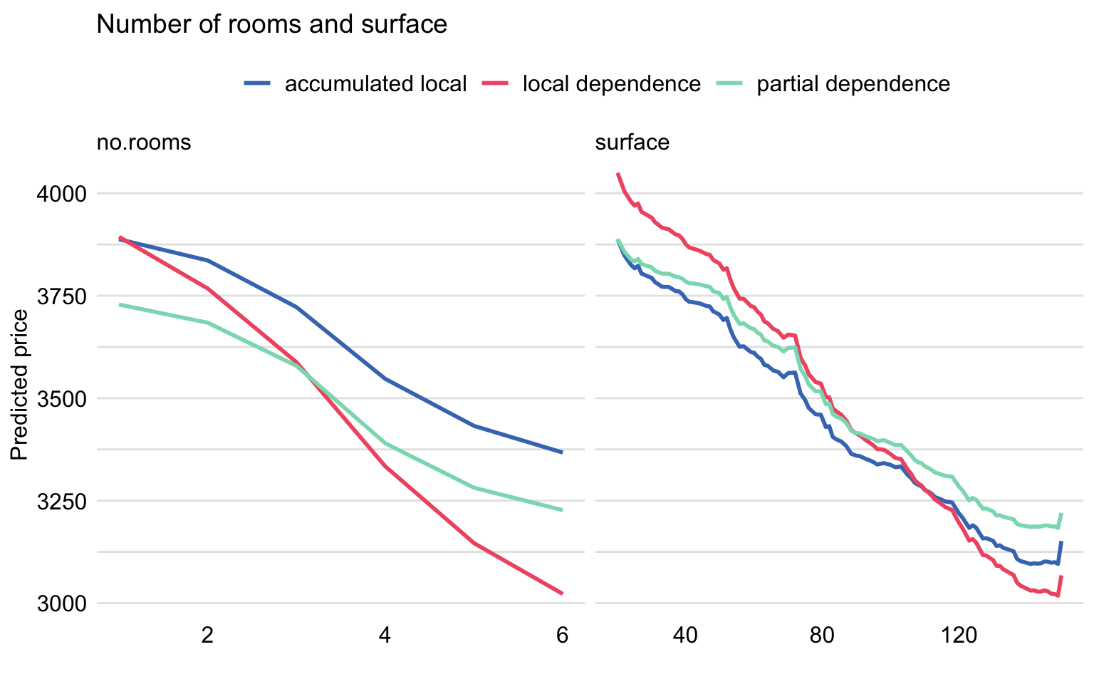
Figure 18.5: Partial-dependence, local-dependence, and accumulated-local profiles for the random forest model for the apartment-prices dataset.

18.5 Pros and cons

The LD and AL profiles, described in this chapter, are useful to summarize the influence of an explanatory variable on a model’s predictions. The profiles are constructed by using the CP profiles introduced in Chapter 10, but they differ in how the CP profiles for individual observations are summarized.

When explanatory variables are independent and there are no interactions in the model, the CP profiles are parallel and their mean, i.e., the PD profile introduced in Chapter 17, adequately summarizes them.

When the model is additive, but an explanatory variable is correlated with some other variables, neither PD nor LD profiles will properly capture the effect of the explanatory variable on the model’s predictions. However, the AL profile will provide a correct summary of the effect.

When there are interactions in the model, none of the profiles will provide a correct assessment of the effect of any explanatory variable involved in the interaction(s). This is because the profiles for the variable will also include the effect of other variables. Comparison of PD, LD, and AL profiles may help in identifying whether there are any interactions in the model and/or whether explanatory variables are correlated. When there are interactions, they may be explored by using a generalization of the PD profiles for two or more dependent variables (Apley and Zhu 2020).

18.6 Code snippets for R

In this section, we present the DALEX package for R, which covers the methods presented in this chapter. In particular, it includes wrappers for functions from the ingredients package (Biecek et al. 2019). Note that similar functionalities can be found in package ALEPlots (Apley 2018) or iml (Molnar, Bischl, and Casalicchio 2018).

For illustration purposes, we use the random forest model apartments_rf (see Section 4.5.2) for the apartment prices dataset (see Section 4.4). Recall that the goal is to predict the price per square meter of an apartment. In our illustration, we focus on two explanatory variables, surface and number of rooms.

We first load the model-object via the archivist hook, as listed in Section 4.5.6. Then we construct the explainer for the model by using the function explain() from the DALEX package (see Section 4.2.6). Note that, beforehand, we have got to load the randomForest package, as the model was fitted by using function randomForest() from this package (see Section 4.2.2) and it is important to have the corresponding predict() function available.

library("DALEX")
library("randomForest")
apartments_rf <- archivist::aread("pbiecek/models/fe7a5")
explainer_apart_rf <- DALEX::explain(model = apartments_rf, 
                             data    = apartments_test[,-1],
                             y       = apartments_test$m2.price, 
                             label   = "Random Forest")

The function that allows the computation of LD and AL profiles in the DALEX package is model_profile(). Its use and arguments were described in Section 17.6. LD profiles are calculated by specifying argument type = "conditional". In the example below, we also use the variables argument to calculate the profile only for the explanatory variables surface and no.rooms. By default, the profile is based on 100 randomly selected observations.

ld_rf <- model_profile(explainer = explainer_apart_rf,
                      type       = "conditional",
                      variables  = c("no.rooms", "surface"))

The resulting object of class “model_profile” contains the LD profiles for both explanatory variables. By applying the plot() function to the object, we obtain separate plots of the profiles.

plot(ld_rf) +
  ggtitle("Local-dependence profiles for no. of rooms and surface", "")

The resulting plot is shown in Figure 18.6. The profiles essentially correspond to those included in Figure 18.5.

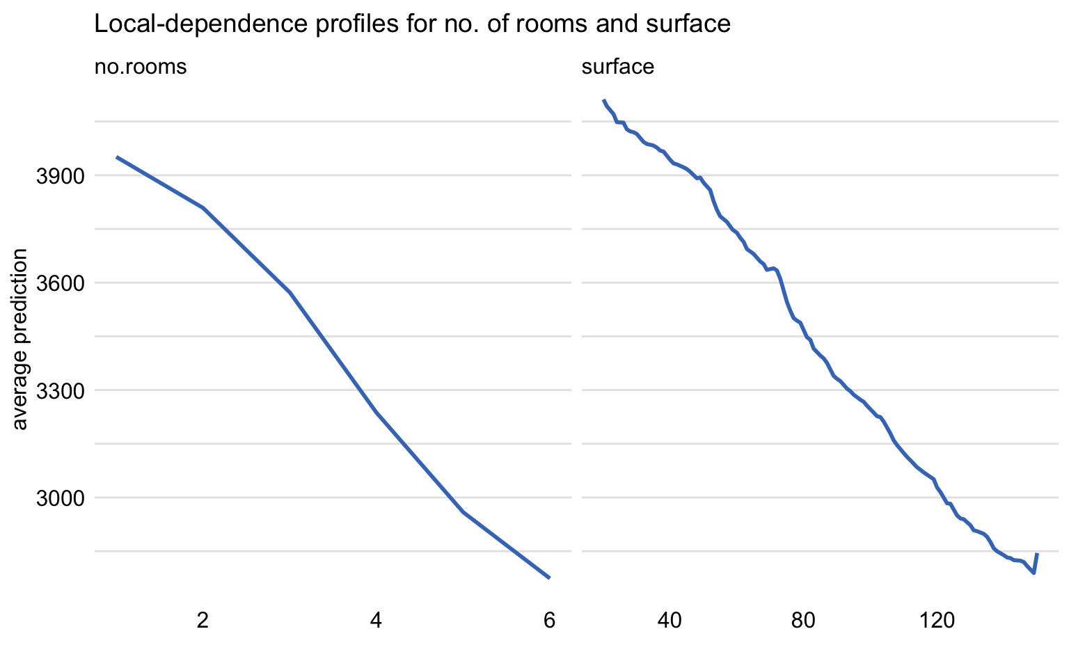
Figure 18.6: Local-dependence profiles for the random forest model and explanatory variables no.rooms and surface for the apartment-prices dataset.

AL profiles are calculated by applying function model_profile() with the additional argument type = "accumulated". In the example below, we also use the variables argument to calculate the profile only for the explanatory variables surface and no.rooms.

al_rf <- model_profile(explainer = explainer_apart_rf,
                            type = "accumulated",
                       variables = c("no.rooms", "surface"))

By applying the plot() function to the object, we obtain separate plots of the AL profiles for no.rooms and surface. They are presented in Figure 18.7. The profiles essentially correspond to those included in Figure 18.5.

plot(al_rf) +
  ggtitle("Accumulated-local profiles for no. of rooms and surface", "")

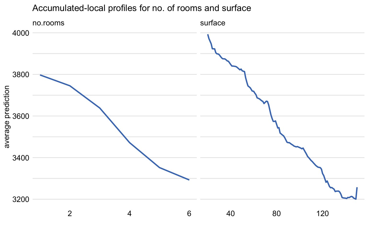
Figure 18.7: Accumulated-local profiles for the random forest model and explanatory variables no.rooms and surface for the apartment-prices dataset.

Function plot() allows including all plots in a single graph. We will show how to apply it in order to obtain Figure 18.5. Toward this end, we have got to create PD profiles first (see Section 17.6). We also modify the labels of the PD, LD, and AL profiles contained in the agr_profiles components of the “model_profile”-class objects created for the different profiles.

pd_rf <- model_profile(explainer = explainer_apart_rf,
                            type = "partial",
                      variables = c("no.rooms", "surface"))
pd_rf$agr_profiles$`_label_` = "partial dependence"
ld_rf$agr_profiles$`_label_` = "local dependence"
al_rf$agr_profiles$`_label_` = "accumulated local"

Subsequently, we simply apply the plot() function to the agr_profiles components of the “model_profile”-class objects for the different profiles (see Section 17.6).

plot(pd_rf, ld_rf, al_rf) 

The resulting plot (not shown) is essentially the same as the one presented in Figure 18.5, with a possible difference due to the use of a different set of (randomly selected) 100 observations from the apartment-prices dataset.

18.7 Code snippets for Python

In this section, we use the dalex library for Python. The package covers all methods presented in this chapter. It is available on pip and GitHub.

For illustration purposes, we use the titanic_rf random forest model for the Titanic data developed in Section 4.3.2. Recall that the model is developed to predict the probability of survival for passengers of Titanic.

In the first step, we create an explainer-object that will provide a uniform interface for the predictive model. We use the Explainer() constructor for this purpose.

import dalex as dx
titanic_rf_exp = dx.Explainer(titanic_rf, X, y, 
                    label = "Titanic RF Pipeline")

The function that allows calculations of LD profiles is model_profile(). It was already introduced in Section 17.7. By defaut, it calculates PD profiles. To obtain LD profiles, the type = 'conditional' should be used.

In the example below, we calculate the LD profile for age and fare by applying the model_profile() function to the explainer-object for the random forest model while specifying type = 'conditional'. Results are stored in the ld_rf.result field.

ld_rf = titanic_rf_exp.model_profile(type = 'conditional')
ld_rf.result['_label_'] = 'LD profiles'
ld_rf.result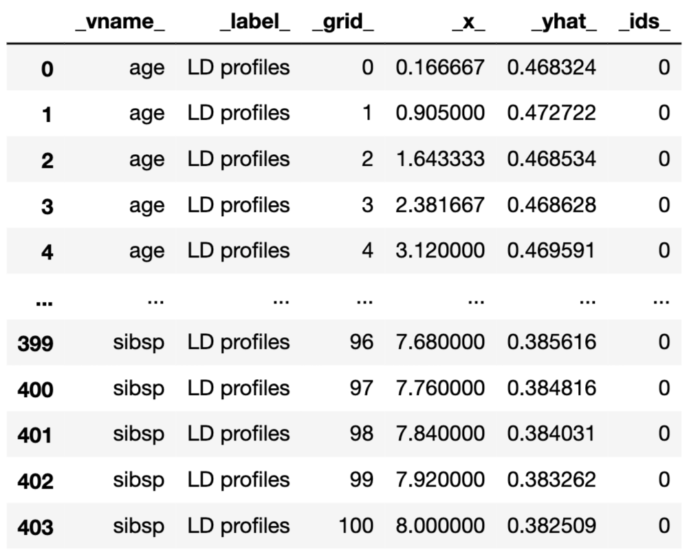

Results can be visualised by using the plot() method. Note that, in the code below, we use the variables argument to display the LD profiles only for age and fare. The resulting plot is presented in Figure 18.8.

ld_rf.plot(variables = ['age', 'fare'])

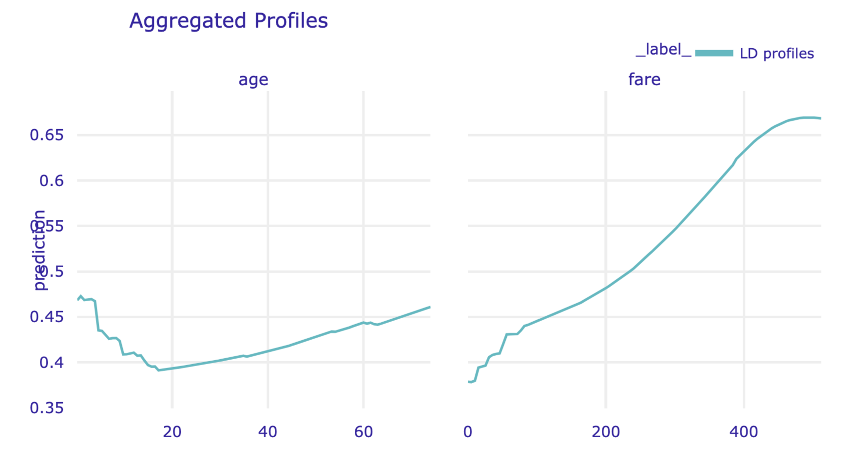
Figure 18.8: Local-dependence profiles for age and fare for the random forest model for the Titanic data, obtained by using the plot() method in Python.

In order to calculate the AL profiles for age and fare, we apply the model_profile() function with the type = 'accumulated' option.

al_rf = titanic_rf_exp.model_profile(type = 'accumulated')
al_rf.result['_label_'] = 'AL profiles'

We can plot AL and LD profiles in a single chart. Toward this end, in the code that follows, we pass the ld_rf object, which contains LD profiles, as the first argument of the plot() method of the al_rf object that includes AL profiles. We also use the variables argument to display the profiles only for age and fare. The resulting plot is presented in Figure 18.9.

al_rf.plot(ld_rf, variables = ['age', 'fare'])

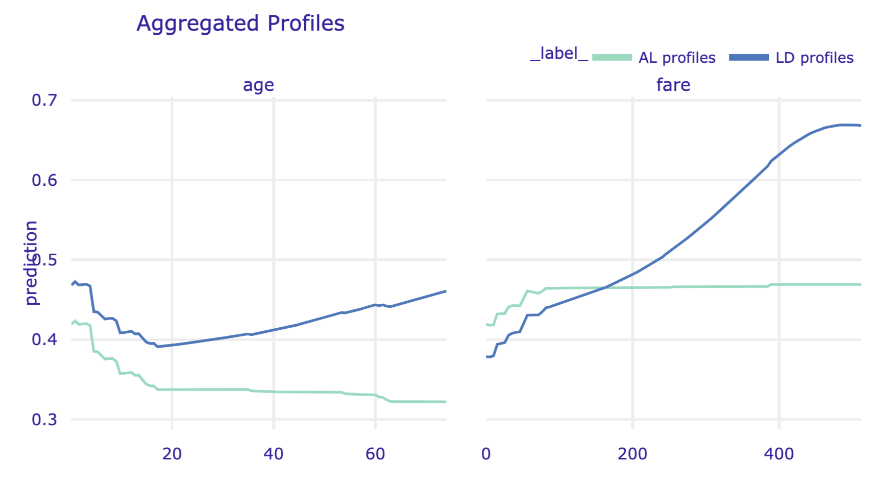
Figure 18.9: Local-dependence and accumulated-local profiles for age and fare for the random forest model for the Titanic data, obtained by using the plot() method in Python.

References

Apley, Dan. 2018. ALEPlot: Accumulated Local Effects (Ale) Plots and Partial Dependence (Pd) Plots. https://CRAN.R-project.org/package=ALEPlot.

Apley, Daniel W., and Jingyu Zhu. 2020. “Visualizing the effects of predictor variables in black box supervised learning models.” Journal of the Royal Statistical Society Series B 82 (4): 1059–86. https://doi.org/10.1111/rssb.12377.

Biecek, Przemyslaw, Hubert Baniecki, Adam Izdebski, and Katarzyna Pekala. 2019. ingredients: Effects and Importances of Model Ingredients. https://github.com/ModelOriented/ingredients.

Molnar, Christoph, Bernd Bischl, and Giuseppe Casalicchio. 2018. “iml: An R package for Interpretable Machine Learning.” Journal of Open Source Software 3 (26): 786. https://doi.org/10.21105/joss.00786.