20 Summary of Dataset-level Exploration
20.1 Introduction
In Part III of the book, we introduced several techniques for global exploration and explanation of a model’s predictions for a set of instances. Each chapter was devoted to a single technique. In practice, these techniques are rarely used separately. Rather, it is more informative to combine different insights offered by each technique into a more holistic overview.
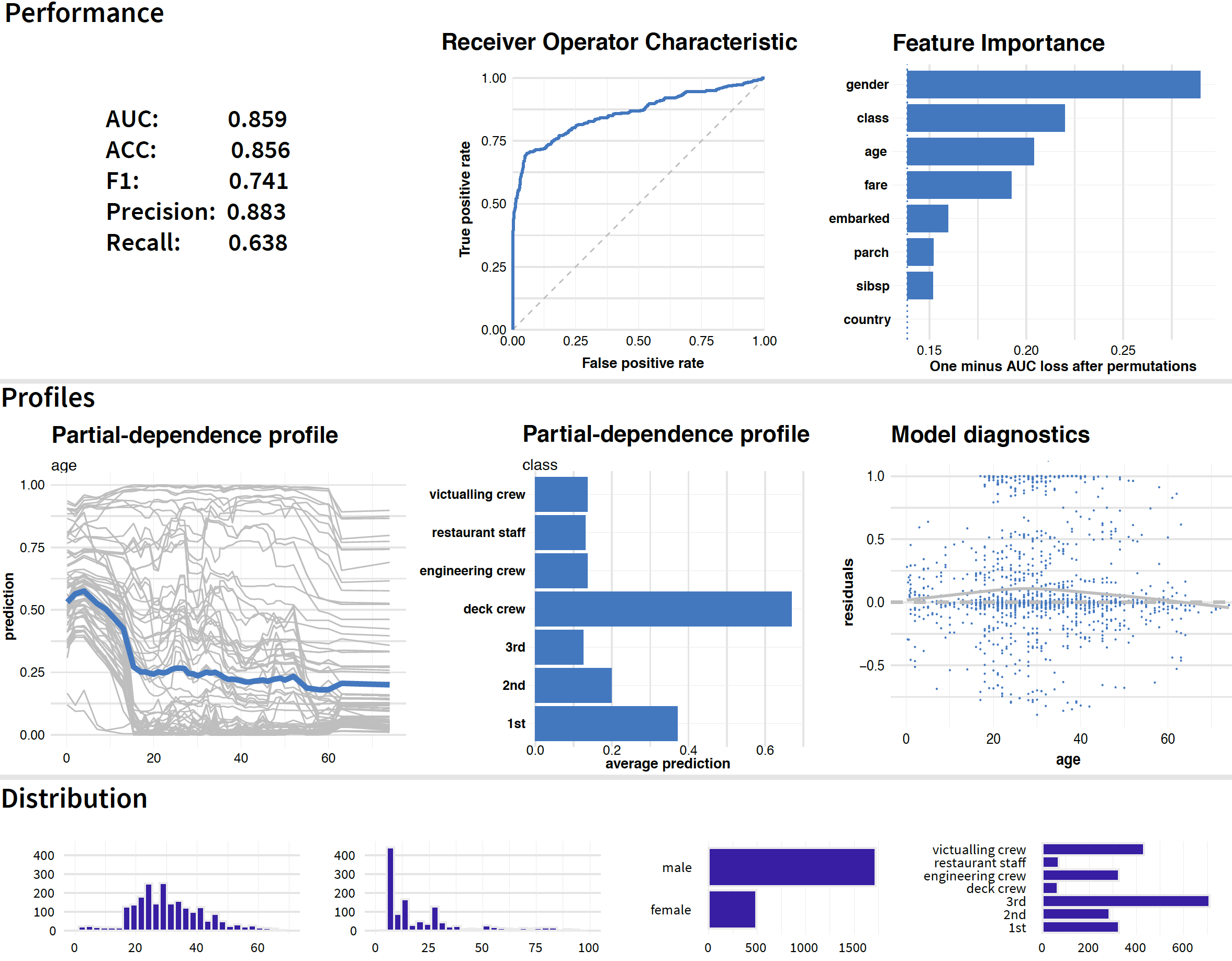
Figure 20.1: Results of dataset-level explanation techniques for the random forest model for the Titanic data.
Figure 20.1 offers a graphical illustration of the idea. The graph includes the results of different dataset-level explanation techniques applied to the random forest model (Section 4.2.2) for the Titanic data (Section 4.1).
The plots in the first row of Figure 20.1 show how good is the model and which variables are the most important. In particular, the first two graphs in that row present measures of the model’s overall performance, as introduced in Chapter 15, along with a graphical summary in the form of the ROC curve. The last plot in the row shows values of the variable-importance measure obtained by the method introduced in Chapter 16. The three graphs indicate a reasonable overall performance of the model and suggest that the most important variables are gender, class, and age.
The two first plots in the second row of Figure 20.1 show partial-dependence (PD) profiles for age (continuous variable) and class (categorical variable). The profile for age suggest that the critical cutoff, from a perspective of the variable’s effect, is around 18 years. The profile for class indicates that, among different travel-classes, the largest effect and chance for survival is associated with the deck crew. The last graph on the right in the second row of Figure 20.1 presents a scatter plot of residuals for age. In the plot, residuals for passengers with age between 20 and 40 years are, on average, slightly larger than for other ages, but the bias is not excessive.
The plots in the third row of Figure 20.1 summarize distributions of (from the left to the right the) age, fare, gender, and class.
Thus, Figure 20.1 illustrates that perspectives offered by different techniques complement each other and, when combined, allow obtaining a more profound insight into the model’s predictive performance.
Figure 20.2 illustrates how the information obtained from model exploration can be used to gain a better understanding of the model and of the domain that is being modelled. Modelling is an iterative process (see Section 2.2), and the more we learn in each iteration, the easier it is to plan and execute the next one.
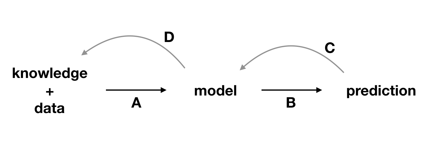
Figure 20.2: Explainability techniques allow strengthening the feedback extracted from a model. A, data and domain knowledge allow building the model. B, predictions are obtained from the model. C, by analyzing the predictions, we learn more about the model. D, better understanding of the model allows better understanding of the data and, sometimes, broadens domain knowledge.
While combining various techniques for dataset-level explanation can provide additional insights, it is worth remembering that the techniques are, indeed, different and their suitability may depend on the problem at hand. This is what we discuss in the remainder of the chapter.
20.2 Exploration on training/testing data
The key element of dataset-level explanatory techniques is the set of observations on which the exploration is performed. Therefore, sometimes these techniques are called dataset-level exploration. This is the terminology that we have adopted.
In the case of machine-learning models, data are often split into a training set and a testing set. Which one should we use for model exploration?
In the case of model-performance assessment, it is natural to evaluate it using an independent testing dataset to minimize the risk of overfitting. However, PD profiles or accumulated-local (AL) profiles can be constructed for both the training and testing datasets. If the model is generalizable, its behavior for the two datasets should be similar. If we notice significant differences in the results for the two datasets, the source of the differences should be examined, as it may be a sign of shifts in variable distributions. Such shifts are called data-drift in the machine learning world.
20.4 Comparison of models (champion-challenger analysis)
One of important applications of the methods presented in Part III of the book is comparison of models.
It appears that different models may offer a similar performance, while basing their predictions on different relations extracted from the same data. Leo Breiman (2001b) refers to this phenomenon as “Rashomon effect”. By comparing models, we can gain important insights that can lead to improvement of one or several of the models. For instance, when comparing a more flexible model with a more rigid one, we can check if they discover similar relationships between the dependent variable and explanatory variables. If they do, this can reassure us that both models have discovered genuine aspects of the data. Sometimes, however, the rigid model may miss a relationship that might have been found by the more flexible one. This could provide, for instance, a suggestion for an improvement of the former. An example of such a case was provided in Chapter 17, in which a linear-regression model was compared to a random forest model for the apartment-prices dataset. The random forest model suggested a U-shaped relationship between the construction year and the price of an apartment, which was missed by the simple linear-regression model.
References
Breiman, Leo. 2001b. “Statistical modeling: The two cultures.” Statistical Science 16 (3): 199–231. https://doi.org/10.1214/ss/1009213726.