9 Local Interpretable Model-agnostic Explanations (LIME)

9.1 Introduction

Break-down (BD) plots and Shapley values, introduced in Chapters 6 and 8, respectively, are most suitable for models with a small or moderate number of explanatory variables.

None of those approaches is well-suited for models with a very large number of explanatory variables, because they usually determine non-zero attributions for all variables in the model. However, in domains like, for instance, genomics or image recognition, models with hundreds of thousands, or even millions, of explanatory (input) variables are not uncommon. In such cases, sparse explanations with a small number of variables offer a useful alternative. The most popular example of such sparse explainers is the Local Interpretable Model-agnostic Explanations (LIME) method and its modifications.

The LIME method was originally proposed by Ribeiro, Singh, and Guestrin (2016). The key idea behind it is to locally approximate a black-box model by a simpler glass-box model, which is easier to interpret. In this chapter, we describe this approach.

9.2 Intuition

The intuition behind the LIME method is explained in Figure 9.1. We want to understand the factors that influence a complex black-box model around a single instance of interest (black cross). The coloured areas presented in Figure 9.1 correspond to decision regions for a binary classifier, i.e., they pertain to a prediction of a value of a binary dependent variable. The axes represent the values of two continuous explanatory variables. The coloured areas indicate combinations of values of the two variables for which the model classifies the observation to one of the two classes. To understand the local behavior of the complex model around the point of interest, we generate an artificial dataset, to which we fit a glass-box model. The dots in Figure 9.1 represent the generated artificial data; the size of the dots corresponds to proximity to the instance of interest. We can fit a simpler glass-box model to the artificial data so that it will locally approximate the predictions of the black-box model. In Figure 9.1, a simple linear model (indicated by the dashed line) is used to construct the local approximation. The simpler model serves as a “local explainer” for the more complex model.

We may select different classes of glass-box models. The most typical choices are regularized linear models like LASSO regression (Tibshirani 1994) or decision trees (Hothorn, Hornik, and Zeileis 2006). Both lead to sparse models that are easier to understand. The important point is to limit the complexity of the models, so that they are easier to explain.

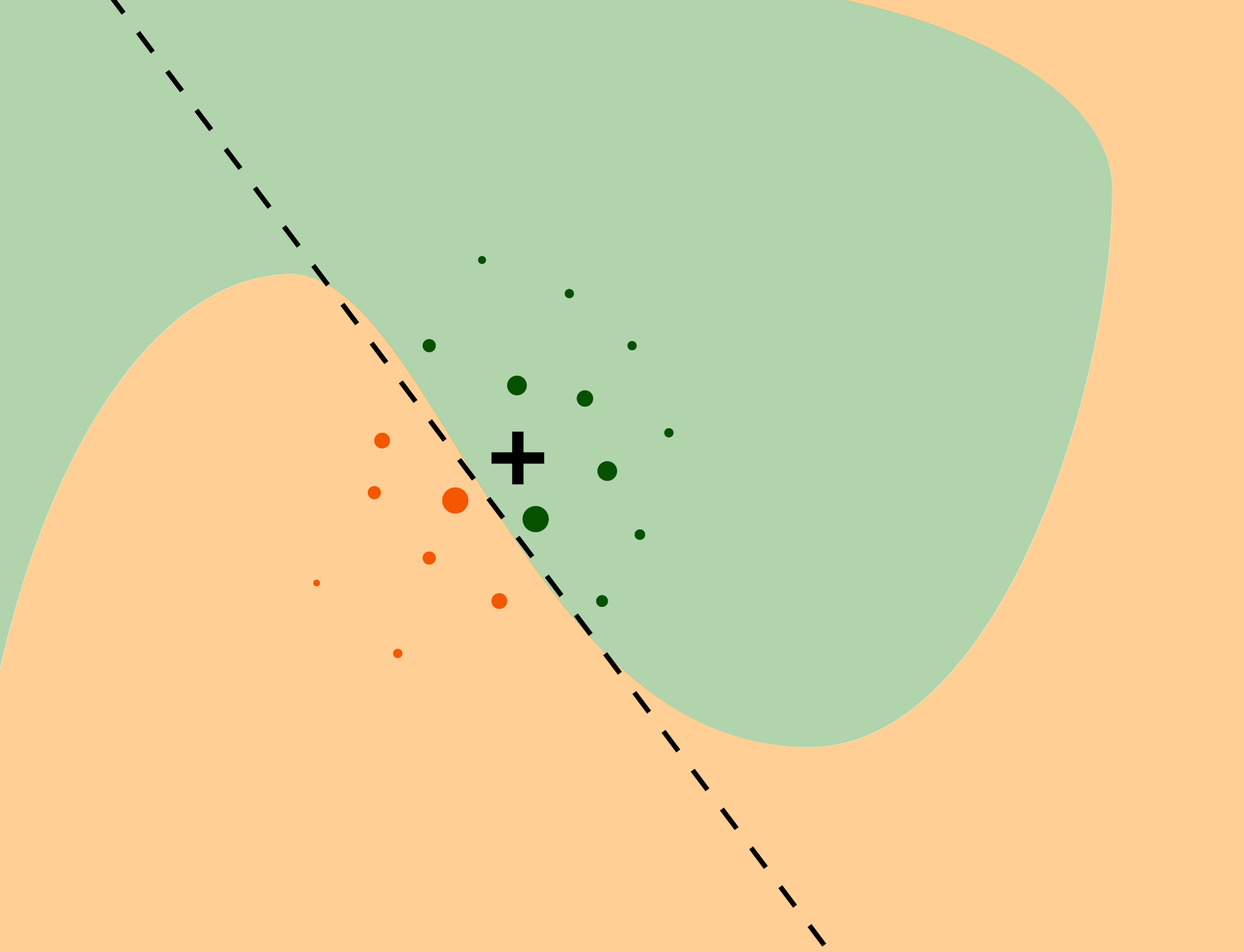
Figure 9.1: The idea behind the LIME approximation with a local glass-box model. The coloured areas correspond to decision regions for a complex binary classification model. The black cross indicates the instance (observation) of interest. Dots correspond to artificial data around the instance of interest. The dashed line represents a simple linear model fitted to the artificial data. The simple model “explains” local behavior of the black-box model around the instance of interest.

9.3 Method

We want to find a model that locally approximates a black-box model \(f()\) around the instance of interest \(\underline{x}_*\). Consider class \(G\) of simple, interpretable models like, for instance, linear models or decision trees. To find the required approximation, we minimize a “loss function”: \[ \hat g = \arg \min_{g \in \mathcal{G}} L\{f, g, \nu(\underline{x}_*)\} + \Omega (g), \] where model \(g()\) belongs to class \(\mathcal{G}\), \(\nu(\underline{x}_*)\) defines a neighborhood of \(\underline{x}_*\) in which approximation is sought, \(L()\) is a function measuring the discrepancy between models \(f()\) and \(g()\) in the neighborhood \(\nu(\underline{x}_*)\), and \(\Omega(g)\) is a penalty for the complexity of model \(g()\). The penalty is used to favour simpler models from class \(\mathcal{G}\). In applications, this criterion is very often simplified by limiting class \(G\) to models with the same complexity, i.e., with the same number of coefficients. In such a situation, \(\Omega(g)\) is the same for each model \(g()\), so it can be omitted in optimization.

Note that models \(f()\) and \(g()\) may operate on different data spaces. The black-box model (function) \(f(\underline{x}):\mathcal X \rightarrow \mathcal R\) is defined on a large, \(p\)-dimensional space \(\mathcal X\) corresponding to the \(p\) explanatory variables used in the model. The glass-box model (function) \(g(\underline{x}):\tilde{ \mathcal X} \rightarrow \mathcal R\) is defined on a \(q\)-dimensional space \(\tilde{ \mathcal X}\) with \(q << p\), often called the “space for interpretable representation”. We will present some examples of \(\tilde{ \mathcal X}\) in the next section. For now we will just assume that some function \(h()\) transforms \(\mathcal X\) into \(\tilde{ \mathcal X}\).

If we limit class \(\mathcal{G}\) to linear models with a limited number, say \(K\), of non-zero coefficients, then the following algorithm may be used to find an interpretable glass-box model \(g()\) that includes \(K\) most important, interpretable, explanatory variables:

Input: x* - observation to be explained
Input: N  - sample size for the glass-box model 
Input: K  - complexity, the number of variables for the glass-box model
Input: similarity - a distance function in the original data space
1. Let x' = h(x*) be a version of x* in the lower-dimensional space
2. for i in 1...N {
3.   z'[i] <- sample_around(x') 
4.   y'[i] <- f(z'[i])       # prediction for new observation z'[i]
5.   w'[i] <- similarity(x', z'[i]) 
6. }
7. return K-LASSO(y', x', w')

In Step 7, K-LASSO(y', x', w') stands for a weighted LASSO linear-regression that selects \(K\) variables based on the new data y' and x' with weights w'.

Practical implementation of this idea involves three important steps, which are discussed in the subsequent subsections.

9.3.1 Interpretable data representation

As it has been mentioned, the black-box model \(f()\) and the glass-box model \(g()\) operate on different data spaces. For example, let us consider a VGG16 neural network (Simonyan and Zisserman 2015) trained on the ImageNet data (Deng et al. 2009). The model uses an image of the size of 244 \(\times\) 244 pixels as input and predicts to which of 1000 potential categories does the image belong to. The original space \(\mathcal X\) is of dimension 3 \(\times\) 244 \(\times\) 244 (three single-color channels (red, green, blue) for a single pixel \(\times\) 244 \(\times\) 244 pixels), i.e., the input space is 178,608-dimensional. Explaining predictions in such a high-dimensional space is difficult. Instead, from the perspective of a single instance of interest, the space can be transformed into superpixels, which are treated as binary features that can be turned on or off. Figure 9.2 (right-hand-side panel) presents an example of 100 superpixels created for an ambiguous picture. Thus, in this case the black-box model \(f()\) operates on space \(\mathcal X=\mathcal{R}^{178608}\), while the glass-box model \(g()\) applies to space \(\tilde{ \mathcal X} = \{0,1\}^{100}\).

It is worth noting that superpixels, based on image segmentation, are frequent choices for image data. For text data, groups of words are frequently used as interpretable variables. For tabular data, continuous variables are often discretized to obtain interpretable categorical data. In the case of categorical variables, combination of categories is often used. We will present examples in the next section.

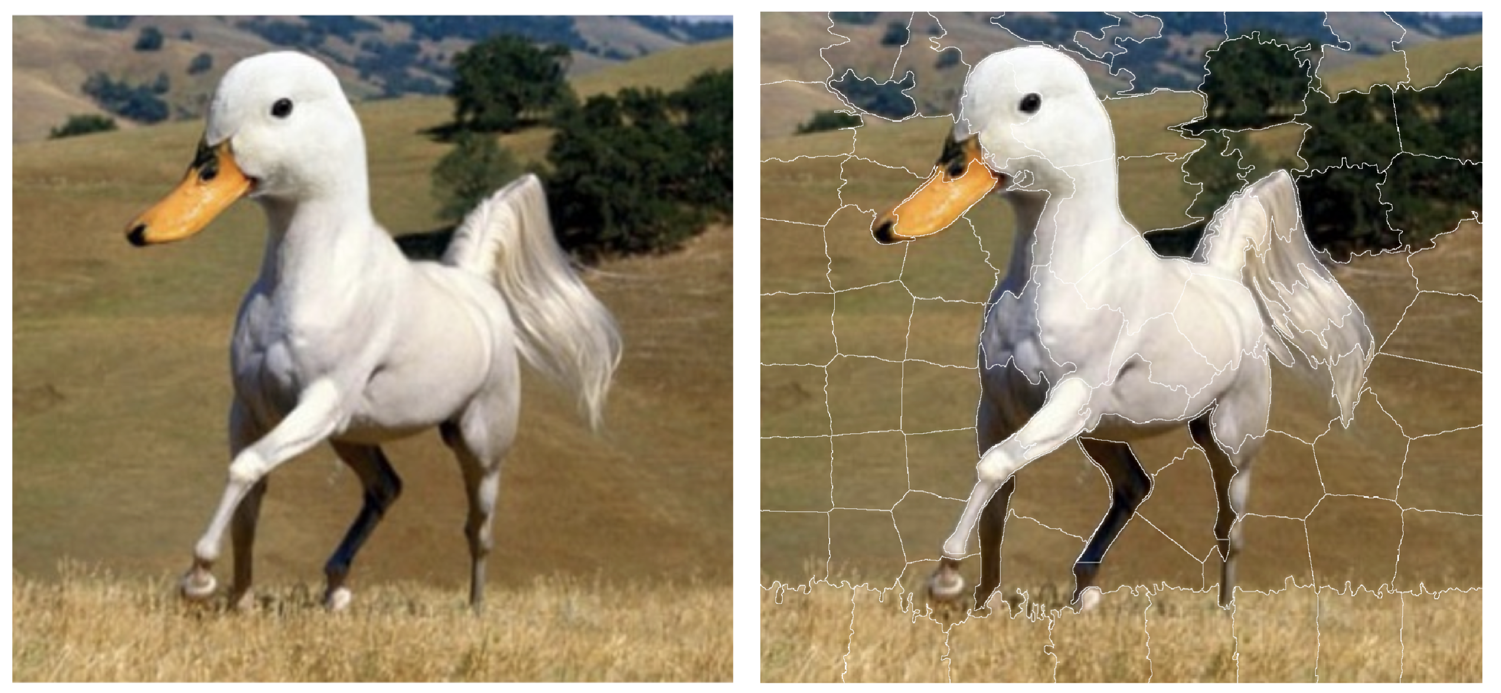
Figure 9.2: The left-hand-side panel shows an ambiguous picture, half-horse and half-duck (source Twitter). The right-hand-side panel shows 100 superpixels identified for this figure.

9.3.2 Sampling around the instance of interest

To develop a local-approximation glass-box model, we need new data points in the low-dimensional interpretable data space around the instance of interest. One could consider sampling the data points from the original dataset. However, there may not be enough points to sample from, because the data in high-dimensional datasets are usually very sparse and data points are “far” from each other. Thus, we need new, artificial data points. For this reason, the data for the development of the glass-box model is often created by using perturbations of the instance of interest.

For binary variables in the low-dimensional space, the common choice is to switch (from 0 to 1 or from 1 to 0) the value of a randomly-selected number of variables describing the instance of interest.

For continuous variables, various proposals have been formulated in different papers. For example, Molnar, Bischl, and Casalicchio (2018) and Molnar (2019) suggest adding Gaussian noise to continuous variables. Pedersen and Benesty (2019) propose to discretize continuous variables by using quantiles and then perturb the discretized versions of the variables. Staniak et al. (2019) discretize continuous variables based on segmentation of local ceteris-paribus profiles (for more information about the profiles, see Chapter 10).

In the example of the duck-horse image in Figure 9.2, the perturbations of the image could be created by randomly excluding some of the superpixels. An illustration of this process is shown in Figure 9.3.

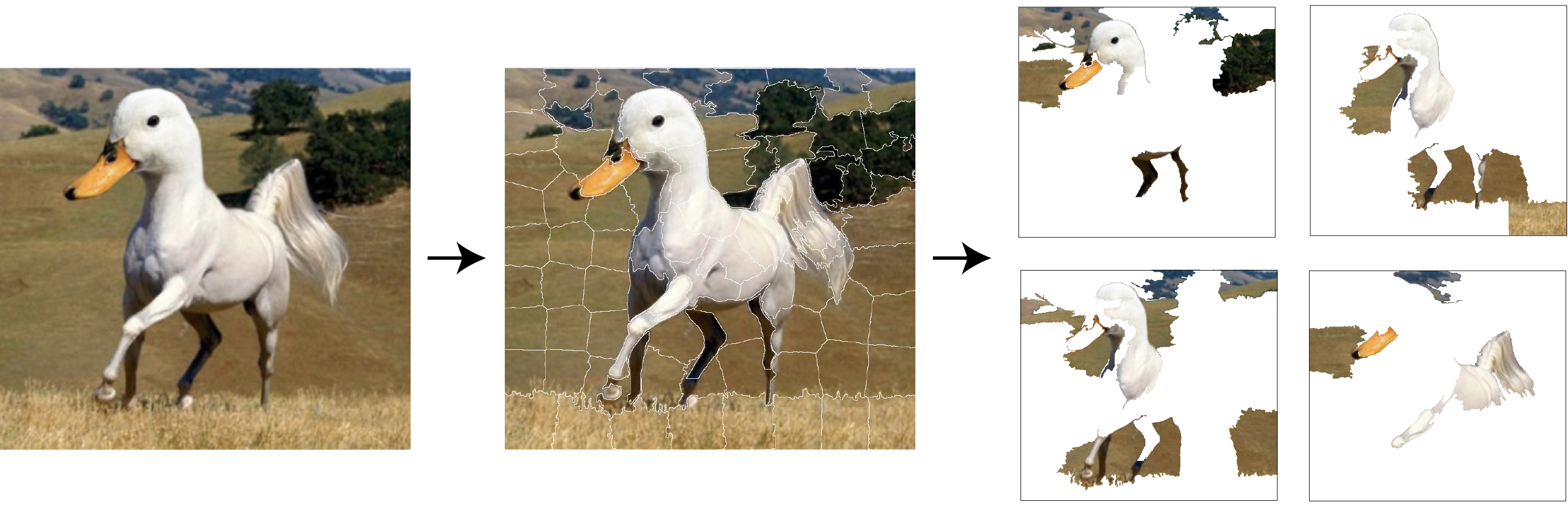
Figure 9.3: The original image (left-hand-side panel) is transformed into a lower-dimensional data space by defining 100 super pixels (panel in the middle). The artificial data are created by using subsets of superpixels (right-hand-side panel).

9.3.3 Fitting the glass-box model

Once the artificial data around the instance of interest have been created, we may attempt to fit an interpretable glass-box model \(g()\) from class \(\mathcal{G}\).

The most common choices for class \(\mathcal{G}\) are generalized linear models. To get sparse models, i.e., models with a limited number of variables, LASSO (least absolute shrinkage and selection operator) (Tibshirani 1994) or similar regularization-modelling techniques are used. For instance, in the algorithm presented in Section 9.3, the K-LASSO method with K non-zero coefficients has been mentioned. An alternative choice are classification-and-regression trees models (Breiman et al. 1984).

For the example of the duck-horse image in Figure 9.2, the VGG16 network provides 1000 probabilities that the image belongs to one of the 1000 classes used for training the network. It appears that the two most likely classes for the image are ‘standard poodle’ (probability of 0.18) and ‘goose’ (probability of 0.15). Figure 9.4 presents LIME explanations for these two predictions. The explanations were obtained with the K-LASSO method, which selected \(K=15\) superpixels that were the most influential from a model-prediction point of view. For each of the selected two classes, the \(K\) superpixels with non-zero coefficients are highlighted. It is interesting to observe that the superpixel which contains the beak is influential for the ‘goose’ prediction, while superpixels linked with the white colour are influential for the ‘standard poodle’ prediction. At least for the former, the influential feature of the plot does correspond to the intended content of the image. Thus, the results of the explanation increase confidence in the model’s predictions.

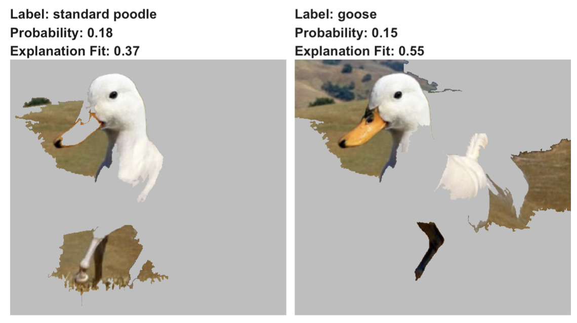
Figure 9.4: LIME for two predictions (‘standard poodle’ and ‘goose’) obtained by the VGG16 network with ImageNet weights for the half-duck, half-horse image. TODO: fix apostrophes!

9.4 Example: Titanic data

Most examples of the LIME method are related to the text or image data. In this section, we present an example of a binary classification for tabular data to facilitate comparisons between methods introduced in different chapters.

Let us consider the random forest model titanic_rf (see Section 4.2.2) and passenger Johnny D (see Section 4.2.5) as the instance of interest for the Titanic data.

First, we have got to define an interpretable data space. One option would be to gather similar variables into larger constructs corresponding to some concepts. For example class and fare variables can be combined into “wealth”, age and gender into “demography”, and so on. In this example, however, we have got a relatively small number of variables, so we will use a simpler data representation in the form of a binary vector. Toward this aim, each variable is dichotomized into two levels. For example, age is transformed into a binary variable with categories “\(\leq\) 15.36” and “>15.36”, class is transformed into a binary variable with categories “1st/2nd/deck crew” and “other”, and so on. Once the lower-dimension data space is defined, the LIME algorithm is applied to this space. In particular, we first have got to appropriately transform data for Johnny D. Subsequently, we generate a new artificial dataset that will be used for K-LASSO approximations of the random forest model. In particular, the K-LASSO method with \(K=3\) is used to identify the three most influential (binary) variables that will provide an explanation for the prediction for Johnny D. The three variables are: age, gender, and class. This result agrees with the conclusions drawn in the previous chapters. Figure 9.5 shows the coefficients estimated for the K-LASSO model.

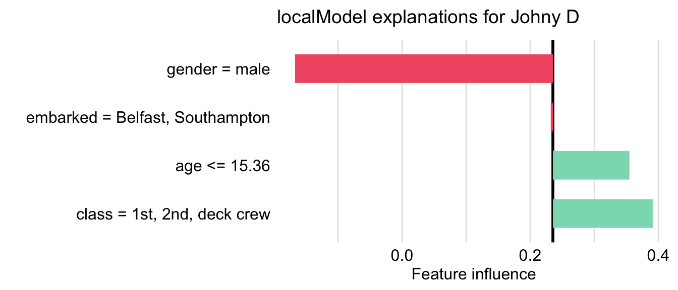
Figure 9.5: LIME method for the prediction for Johnny D for the random forest model titanic_rf and the Titanic data. Presented values are the coefficients of the K-LASSO model fitted locally to the predictions from the original model.

9.5 Pros and cons

As mentioned by Ribeiro, Singh, and Guestrin (2016), the LIME method

• is model-agnostic, as it does not imply any assumptions about the black-box model structure;
• offers an interpretable representation, because the original data space is transformed (for instance, by replacing individual pixels by superpixels for image data) into a more interpretable, lower-dimension space;
• provides local fidelity, i.e., the explanations are locally well-fitted to the black-box model.

The method has been widely adopted in the text and image analysis, partly due to the interpretable data representation. In that case, the explanations are delivered in the form of fragments of an image/text, and users can easily find the justification of such explanations. The underlying intuition for the method is easy to understand: a simpler model is used to approximate a more complex one. By using a simpler model, with a smaller number of interpretable explanatory variables, predictions are easier to explain. The LIME method can be applied to complex, high-dimensional models.

There are several important limitations, however. For instance, as mentioned in Section 9.3.2, there have been various proposals for finding interpretable representations for continuous and categorical explanatory variables in case of tabular data. The issue has not been solved yet. This leads to different implementations of LIME, which use different variable-transformation methods and, consequently, that can lead to different results.

Another important point is that, because the glass-box model is selected to approximate the black-box model, and not the data themselves, the method does not control the quality of the local fit of the glass-box model to the data. Thus, the latter model may be misleading.

Finally, in high-dimensional data, data points are sparse. Defining a “local neighborhood” of the instance of interest may not be straightforward. Importance of the selection of the neighborhood is discussed, for example, by Alvarez-Melis and Jaakkola (2018). Sometimes even slight changes in the neighborhood strongly affect the obtained explanations.

To summarize, the most useful applications of LIME are limited to high-dimensional data for which one can define a low-dimensional interpretable data representation, as in image analysis, text analysis, or genomics.

9.6 Code snippets for R

LIME and its variants are implemented in various R and Python packages. For example, lime (Pedersen and Benesty 2019) started as a port of the LIME Python library (Lundberg 2019), while localModel (Staniak et al. 2019), and iml (Molnar, Bischl, and Casalicchio 2018) are separate packages that implement a version of this method entirely in R.

Different implementations of LIME offer different algorithms for extraction of interpretable features, different methods for sampling, and different methods of weighting. For instance, regarding transformation of continuous variables into interpretable features, lime performs global discretization using quartiles, localModel performs local discretization using ceteris-paribus profiles (for more information about the profiles, see Chapter 10), while iml works directly on continuous variables. Due to these differences, the packages yield different results (explanations).

Also, lime, localModel, and iml use different functions to implement the LIME method. Thus, we will use the predict_surrogate() method from the DALEXtra package. The function offers a uniform interface to the functions from the three packages.

In what follows, for illustration purposes, we use the titanic_rf random forest model for the Titanic data developed in Section 4.2.2. Recall that it is developed to predict the probability of survival from the sinking of the Titanic. Instance-level explanations are calculated for Johnny D, an 8-year-old passenger that travelled in the first class. We first retrieve the titanic_rf model-object and the data frame for Johnny D via the archivist hooks, as listed in Section 4.2.7. We also retrieve the version of the titanic data with imputed missing values.

titanic_imputed <- archivist::aread("pbiecek/models/27e5c")
titanic_rf <- archivist:: aread("pbiecek/models/4e0fc")
johnny_d <- archivist:: aread("pbiecek/models/e3596")

  class gender age sibsp parch fare    embarked
1   1st   male   8     0     0   72 Southampton

Then we construct the explainer for the model by using the function explain() from the DALEX package (see Section 4.2.6). We also load the randomForest package, as the model was fitted by using function randomForest() from this package (see Section 4.2.2) and it is important to have the corresponding predict() function available.

library("randomForest")
library("DALEX")
titanic_rf_exp <- DALEX::explain(model = titanic_rf,  
                        data = titanic_imputed[, -9],
                           y = titanic_imputed$survived == "yes", 
                       label = "Random Forest")

9.6.1 The lime package

The key functions in the lime package are lime(), which creates an explanation, and explain(), which evaluates explanations. As mentioned earlier, we will apply the predict_surrogate() function from the DALEXtra package to access the functions via an interface that is consistent with the approach used in the previous chapters.

The predict_surrogate() function requires two arguments: explainer, which specifies the name of the explainer-object created with the help of function explain() from the DALEX package, and new_observation, which specifies the name of the data frame for the instance for which prediction is of interest. An additional, important argument is type that indicates the package with the desired implementation of the LIME method: either "localModel" (default), "lime", or "iml". In case of the lime-package implementation, we can specify two additional arguments: n_features to indicate the maximum number (\(K\)) of explanatory variables to be selected by the K-LASSO method, and n_permutations to specify the number of artifical data points to be sampled for the local-model approximation.

In the code below, we apply the predict_surrogate() function to the explainer-object for the random forest model titanic_rf and data for Johnny D. Additionally, we specify that the K-LASSO method should select no more than n_features=3 explanatory variables based on a fit to n_permutations=1000 sampled data points. Note that we use the set.seed() function to ensure repeatability of the sampling.

set.seed(1)
library("DALEXtra")
library("lime")
model_type.dalex_explainer <- DALEXtra::model_type.dalex_explainer
predict_model.dalex_explainer <- DALEXtra::predict_model.dalex_explainer

lime_johnny <- predict_surrogate(explainer = titanic_rf_exp, 
                  new_observation = johnny_d, 
                  n_features = 3, 
                  n_permutations = 1000,
                  type = "lime")

The contents of the resulting object can be printed out in the form of a data frame with 11 variables.

(as.data.frame(lime_johnny))

##   model_type case  model_r2 model_intercept model_prediction feature
## 1 regression    1 0.6826437       0.5541115        0.4784804  gender
## 2 regression    1 0.6826437       0.5541115        0.4784804     age
## 3 regression    1 0.6826437       0.5541115        0.4784804   class
##   feature_value feature_weight  feature_desc                 data
## 1             2     -0.4038175 gender = male 1, 2, 8, 0, 0, 72, 4
## 2             8      0.1636630     age <= 22 1, 2, 8, 0, 0, 72, 4
## 3             1      0.1645234   class = 1st 1, 2, 8, 0, 0, 72, 4
##   prediction
## 1      0.422
## 2      0.422
## 3      0.422

The output includes column case that provides indices of observations for which the explanations are calculated. In our case there is only one index equal to 1, because we asked for an explanation for only one observation, Johnny D. The feature column indicates which explanatory variables were given non-zero coefficients in the K-LASSO method. The feature_value column provides information about the values of the original explanatory variables for the observations for which the explanations are calculated. On the other hand, the feature_desc column indicates how the original explanatory variable was transformed. Note that the applied implementation of the LIME method dichotomizes continuous variables by using quartiles. Hence, for instance, age for Johnny D was transformed into a binary variable age <= 22.

Column feature_weight provides the estimated coefficients for the variables selected by the K-LASSO method for the explanation. The model_intercept column provides of the value of the intercept. Thus, the linear combination of the transformed explanatory variables used in the glass-box model approximating the random forest model around the instance of interest, Johnny D, is given by the following equation (see Section 2.5):

\[ \hat p_{lime} = 0.55411 - 0.40381 \cdot 1_{male} + 0.16366 \cdot 1_{age <= 22} + 0.16452 \cdot 1_{class = 1st} = 0.47848, \] where \(1_A\) denotes the indicator variable for condition \(A\). Note that the computed value corresponds to the number given in the column model_prediction in the printed output.

By applying the plot() function to the object containing the explanation, we obtain a graphical presentation of the results.

plot(lime_johnny)

The resulting plot is shown in Figure 9.6. The length of the bar indicates the magnitude (absolute value), while the color indicates the sign (red for negative, blue for positive) of the estimated coefficient.

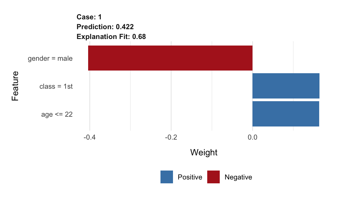
Figure 9.6: Illustration of the LIME-method results for the prediction for Johnny D for the random forest model titanic_rf and the Titanic data, generated by the lime package.

9.6.2 The localModel package

The key function of the localModel package is the individual_surrogate_model() function that fits the local glass-box model. The function is applied to the explainer-object obtained with the help of the DALEX::explain() function (see Section 4.2.6). As mentioned earlier, we will apply the predict_surrogate() function from the DALEXtra package to access the functions via an interface that is consistent with the approach used in the previous chapters. To choose the localModel-implementation of LIME, we set argument type="localMode" (see Section 9.6.1). In that case, the method accepts, apart from the required arguments explainer and new_observation, two additional arguments: size, which specifies the number of artificial data points to be sampled for the local-model approximation, and seed, which sets the seed for the random-number generation allowing for a repeatable execution.

In the code below, we apply the predict_surrogate() function to the explainer-object for the random forest model titanic_rf and data for Johnny D. Additionally, we specify that 1000 data points are to be sampled and we set the random-number-generation seed.

library("localModel")
locMod_johnny <- predict_surrogate(explainer = titanic_rf_exp, 
                  new_observation = johnny_d, 
                  size = 1000, 
                  seed = 1,
                  type = "localModel")

The resulting object is a data frame with seven variables (columns). For brevity, we only print out the first three variables.

locMod_johnny[,1:3]

##     estimated                        variable original_variable
## 1  0.23530947                    (Model mean)                  
## 2  0.30331646                     (Intercept)                  
## 3  0.06004988                   gender = male            gender
## 4 -0.05222505                    age <= 15.36               age
## 5  0.20988506     class = 1st, 2nd, deck crew             class
## 6  0.00000000 embarked = Belfast, Southampton          embarked

The printed output includes column estimated that contains the estimated coefficients of the LASSO regression model, which is used to approximate the predictions from the random forest model. Column variable provides the information about the corresponding variables, which are transformations of original_variable. Note that the version of LIME, implemented in the localModel package, dichotomizes continuous variables by using ceteris-paribus profiles (for more information about the profiles, see Chapter 10). The profile for variable age for Johnny D can be obtained by using function plot_interpretable_feature(), as shown below.

plot_interpretable_feature(locMod_johnny, "age")

The resulting plot is presented in Figure 9.7. The profile indicates that the largest drop in the predicted probability of survival is observed when the value of age increases beyond about 15 years. Hence, in the output of the predict_surrogate() function, we see a binary variable age <= 15.36, as Johnny D was 8 years old.

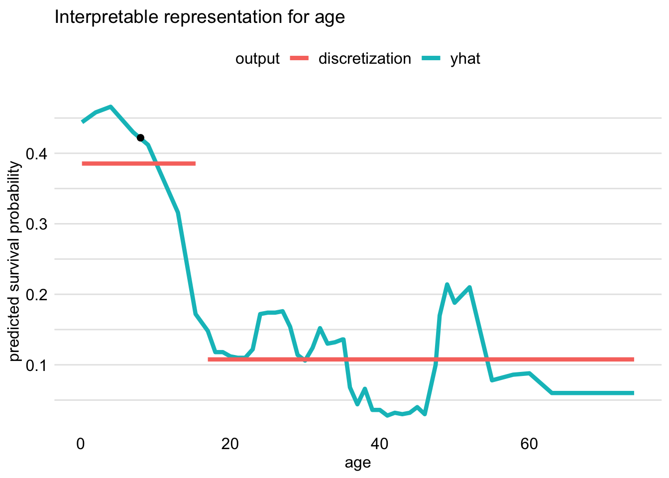
Figure 9.7: Discretization of the age variable for Johnny D based on the ceteris-paribus profile. The optimal change-point is around 15 years of age.

By applying the generic plot() function to the object containing the LIME-method results, we obtain a graphical representation of the results.

plot(locMod_johnny)

The resulting plot is shown in Figure 9.8. The lengths of the bars indicate the magnitude (absolute value) of the estimated coefficients of the LASSO logistic regression model. The bars are placed relative to the value of the mean prediction, 0.235.

Figure 9.8: Illustration of the LIME-method results for the prediction for Johnny D for the random forest model titanic_rf and the Titanic data, generated by the localModel package.

9.6.3 The iml package

The key functions of the iml package are Predictor$new(), which creates an explainer, and LocalModel$new(), which develops the local glass-box model. The main arguments of the Predictor$new() function are model, which specifies the model-object, and data, the data frame used for fitting the model. As mentioned earlier, we will apply the predict_surrogate() function from the DALEXtra package to access the functions via an interface that is consistent with the approach used in the previous chapters. To choose the iml-implementation of LIME, we set argument type="iml" (see Section 9.6.1). In that case, the method accepts, apart from the required arguments explainerand new_observation, an additional argument k that specifies the number of explanatory variables included in the local-approximation model.

library("DALEXtra")
library("iml")
iml_johnny <- predict_surrogate(explainer = titanic_rf_exp, 
                  new_observation = johnny_d, 
                  k = 3, 
                  type = "iml")

The resulting object includes data frame results with seven variables that provides results of the LASSO logistic regression model which is used to approximate the predictions of the random forest model. For brevity, we print out selected variables.

iml_johnny$results[,c(1:5,7)]

##            beta x.recoded      effect x.original     feature .class
## 1 -0.1992616770         1 -0.19926168        1st   class=1st     no
## 2  1.6005493672         1  1.60054937       male gender=male     no
## 3 -0.0002111346        72 -0.01520169         72        fare     no
## 4  0.1992616770         1  0.19926168        1st   class=1st    yes
## 5 -1.6005493672         1 -1.60054937       male gender=male    yes
## 6  0.0002111346        72  0.01520169         72        fare    yes

The printed output includes column beta that provides the estimated coefficients of the local-approximation model. Note that two sets of three coefficients (six in total) are given, corresponding to the prediction of the probability of death (column .class assuming value no, corresponding to the value "no" of the survived dependent-variable) and survival (.class asuming value yes). Column x.recoded contains the information about the value of the corresponding transformed (interpretable) variable. The value of the original explanatory variable is given in column x.original, with column feature providing the information about the corresponding variable. Note that the implemented version of LIME does not transform continuous variables. Categorical variables are dichotomized, with the resulting binary variable assuming the value of 1 for the category observed for the instance of interest and 0 for other categories.

The effect column provides the product of the estimated coefficient (from column beta) and the value of the interpretable covariate (from column x.recoded) of the model approximating the random forest model.

By applying the generic plot() function to the object containing the LIME-method results, we obtain a graphical representation of the results.

plot(iml_johnny) 

The resulting plot is shown in Figure 9.9. It shows values of the two sets of three coefficients for both types of predictions (probability of death and survival).

plot(iml_johnny) 

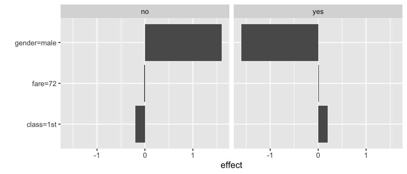
Figure 9.9: Illustration of the LIME-method results for the prediction for Johnny D for the random forest model titanic_rf and the Titanic data, generated by the iml package.

It is worth noting that age, gender, and class are correlated. For instance, crew members are only adults and mainly men. This is probably the reason why the three packages implementing the LIME method generate slightly different explanations for the model prediction for Johnny D.

9.7 Code snippets for Python

In this section, we use the lime library for Python, which is probably the most popular implementation of the LIME method (Ribeiro, Singh, and Guestrin 2016). The lime library requires categorical variables to be encoded in a numerical format. This requires some additional work with the data. Therefore, below we will show you how to use this method in Python step by step.

For illustration purposes, we use the random forest model for the Titanic data. Instance-level explanations are calculated for Henry, a 47-year-old passenger that travelled in the 1st class.

In the first step, we read the Titanic data and encode categorical variables. In this case, we use the simplest encoding for gender, class, and embarked, i.e., the label-encoding.

import dalex as dx

titanic = dx.datasets.load_titanic()
X = titanic.drop(columns='survived')
y = titanic.survived

from sklearn import preprocessing
le = preprocessing.LabelEncoder()

X['gender']   = le.fit_transform(X['gender'])
X['class']    = le.fit_transform(X['class'])
X['embarked'] = le.fit_transform(X['embarked'])

In the next step we train a random forest model.

from sklearn.ensemble import RandomForestClassifier as rfc
titanic_fr = rfc()
titanic_fr.fit(X, y)

It is time to define the observation for which model prediction will be explained. We write Henry’s data into pandas.Series object.

import pandas as pd
henry = pd.Series([1, 47.0, 0, 1, 25.0, 0, 0], 
                  index =['gender', 'age', 'class', 'embarked',
                          'fare', 'sibsp', 'parch']) 

The lime library explains models that operate on images, text, or tabular data. In the latter case, we have to use the LimeTabularExplainer module.

from lime.lime_tabular import LimeTabularExplainer 
explainer = LimeTabularExplainer(X, 
                      feature_names=X.columns, 
                      class_names=['died', 'survived'], 
                      discretize_continuous=False, 
                      verbose=True)

The result is an explainer that can be used to interpret a model around specific observations. In the following example, we explain the behaviour of the model for Henry. The explain_instance() method finds a local approximation with an interpretable linear model. The result can be presented graphically with the show_in_notebook() method.

lime = explainer.explain_instance(henry, titanic_fr.predict_proba)
lime.show_in_notebook(show_table=True)

The resulting plot is shown in Figure 9.10.

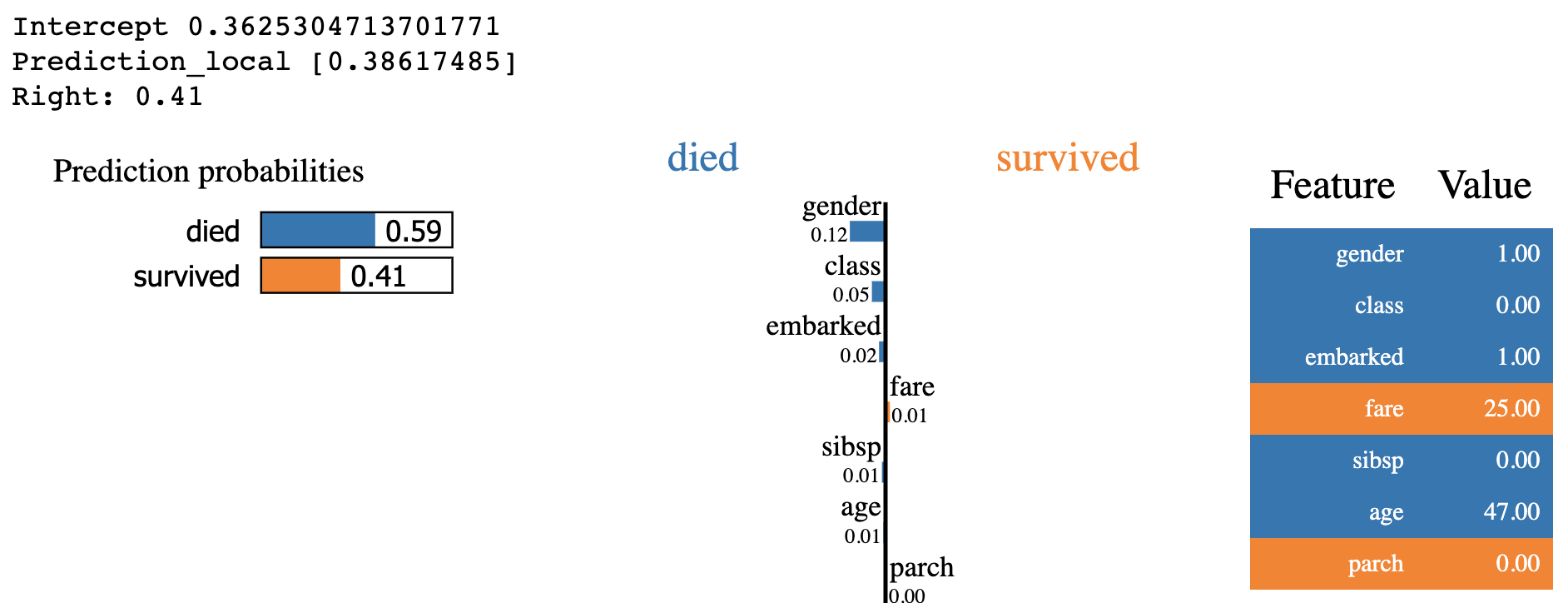
Figure 9.10: A plot of LIME model values for the random forest model and passenger Henry for the Titanic data.

References

Alvarez-Melis, David, and Tommi S. Jaakkola. 2018. “On the Robustness of Interpretability Methods.” ICML Workshop on Human Interpretability in Machine Learning (WHI 2018), June. http://arxiv.org/abs/1806.08049.

Breiman, L., J. H. Friedman, R. A. Olshen, and C. J. Stone. 1984. Classification and Regression Trees. Monterey, CA: Wadsworth; Brooks.

Deng, J., W. Dong, R. Socher, L. Li, Kai Li, and Li Fei-Fei. 2009. “ImageNet: A large-scale hierarchical image database.” In 2009 Ieee Conference on Computer Vision and Pattern Recognition, 248–55. Los Alamitos, CA, USA: IEEE Computer Society. https://doi.org/10.1109/cvpr.2009.5206848.

Hothorn, Torsten, Kurt Hornik, and Achim Zeileis. 2006. “Unbiased Recursive Partitioning: A Conditional Inference Framework.” Journal of Computational and Graphical Statistics 15 (3): 651–74.

Lundberg, Scott. 2019. SHAP (SHapley Additive exPlanations). https://github.com/slundberg/shap.

Molnar, Christoph. 2019. Interpretable Machine Learning: A Guide for Making Black Box Models Explainable.

Molnar, Christoph, Bernd Bischl, and Giuseppe Casalicchio. 2018. “iml: An R package for Interpretable Machine Learning.” Journal of Open Source Software 3 (26): 786. https://doi.org/10.21105/joss.00786.

Pedersen, Thomas Lin, and Michaël Benesty. 2019. lime: Local Interpretable Model-Agnostic Explanations. https://CRAN.R-project.org/package=lime.

Ribeiro, Marco Tulio, Sameer Singh, and Carlos Guestrin. 2016. “"Why should I trust you?": Explaining the Predictions of Any Classifier.” In Proceedings of the 22nd ACM SIGKDD International Conference on Knowledge Discovery and Data Mining, Kdd San Francisco, ca, 1135–44. New York, NY: Association for Computing Machinery.

Simonyan, Karen, and Andrew Zisserman. 2015. “Very Deep Convolutional Networks for Large-Scale Image Recognition.” In International Conference on Learning Representations. San Diego, CA: ICLR 2015.

Staniak, Mateusz, Przemyslaw Biecek, Krystian Igras, and Alicja Gosiewska. 2019. localModel: LIME-Based Explanations with Interpretable Inputs Based on Ceteris Paribus Profiles. https://CRAN.R-project.org/package=localModel.

Tibshirani, Robert. 1994. “Regression Shrinkage and Selection via the lasso.” Journal of the Royal Statistical Society, Series B 58: 267–88.